Week 4- Rolling operation

OBJECTIVE: 

To simulate the rolling operation on a workpiece made of copper by increasing the length of the workpiece by 60 mm and decreasing its size on both sides by 8 mm. Run the simulation for 14 steps by ensuring that the edge of the workpiece is displaced by 90 mm.

To find out the following results:

1. Equivalent stress for the whole setup.
2. Equivalent elastic strain for the workpiece.
3. Directional Deformation in the Z-axis for the workpiece.
4. Prove that the workpiece has displaced 90 mm.

1. THEORY:

ROLLING:

Rolling is the process of reducing the thickness or changing the cross-section of a long strip by compressive forces applied through a set of rolls. In addition to flat rolling, Shape rolling is used to make products with various cross-sections. Products made by rolling include (a)Plate, Sheet, Foil, Rod, Seamless pipe, and Tubing, (b) Shape rolled products like I-section, C-section and Various Structural shapes, (c) Bars of the various cross-sections. 

Other rolling operations include ring rolling and thread rolling.

Rolling may be carried out at room temperature(cold rolling) or elevated temperatures (hot-rolling). The process involves several material and process variables, including roll diameter (relative to material thickness), reduction per pass, speed, lubrication, and temperature, spreading, bending and flattering are important considerations for controlling the dimensional accuracy of the rolled stock.

                   

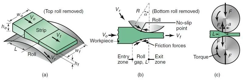
Fig 1.2 Schematic illustration of (a) The flat rolling process (b) Friction forces acting on strip surfaces (c) Roll Force "F" and Torque "T" acting on the rolls.

A schematic illustration of the flat-rolling process is shown in Fig. 1.2a. A metal strip of thickness h₀ enters the roll gap and is reduced to thickness h_f by a pair of rotating rolls, each powered individually by electric motors. The surface speed of the rolls is Vr. The velocity of the strip increases from its entry value of V₀ as it moves through the roll gap; the velocity of the strip is highest at the exit from the roll gap and is denoted as V_f. The metal accelerates in the roll gap in the same manner as an incompressible fluid flowing through a converging channel. Because the surface speed of the rigid roll is constant, there is relative sliding between the roll and the strip along the arc of contact in the roll gap, L. At one point along the contact length (called the neutral point or no-slip point) the velocity of the strip is the same as that of the roll. To the left of this point, the roll moves faster than the strip; to the right of this point, the strip moves faster than the roll. Consequently, the frictional forces which oppose motion between two sliding bodies act on the strip as shown in Fig. 1.1b.

The rolls pull the material into the roll gap through a net frictional force on the material. Thus, the net frictional force must be to the right in Fig. 1.1b. This also means that the frictional force to the left of the neutral point must be higher than the friction force to the right. Although friction is necessary for rolling materials, energy is dissipated in overcoming friction. Thus, increasing friction also increases rolling forces and power requirements. Furthermore, high friction could damage the surface of the rolled product. Thus, a compromise is made in practice: Low and controlled friction is induced in rolling through the use of effective lubricants.

The maximum possible draft is defined as the difference between the initial and final strip thicknesses, or (h_o – h_f). It can be shown that this quantity is a function of the roll radius, R, and the coefficient of friction, between the strip and the roll by the following relationship:

ho−hf=μ2Rho-hf=μ2R

Thus, as expected, the higher the friction and the larger the roll radius, the greater the maximum possible draft becomes.

In rolling plates and sheets with high width-to-thickness ratios, the width of the strip remains effectively constant during rolling. However, with smaller ratios (such as a strip with a square cross-section), its width increases significantly as it passes through the rolls. This increase in width is called spreading. It can be shown that spreading increases with (a) decreasing width-to-thickness ratio of the entering strip (because of reduction in the width constraint), (b) increasing friction, and (c) decreasing ratio of the roll radius to the strip thickness. The last two effects are due to the increased longitudinal constraint of the material flow in the roll gap. Spreading can be prevented also by using additional rolls (with vertical axes) in contact with the edges of the rolled product in the roll gap (edger mills), thus providing a physical constraint to spreading.\

2. STEPS FOR PERFORMING ANALYSIS:

1. Open ANSYS workbench.

2. Select the static structural module.

3. Select the proper Engineering data card.

4. Import geometry.

5. Open Mechanical model.

6. Give proper connections (contacts and joints).

7. Generate mesh.

8. Set Analysis Setting as given.

9. Insert output request

10. Analyze Result.

Analysis Setup:

3. Geometry:

                   

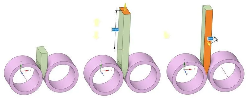
                                 a. Imported model.                b.Length increased to 60 mm.             c. Width decreased on both sides by 8 mm.

The given 3D model of copper rolling assembly is imported into SpaceClaim. The length of the workpiece is increased to 60 mm and the width is decreased on both sides by 8 mm.

4. Meshed Model:

                                                                               

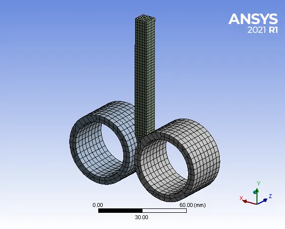
• Details:

1. Body Sizing (Workpiece) = 2mm
2. Global Sizing = 4mm
3. No of Nodes = 13149
4. No of Elements = 2333

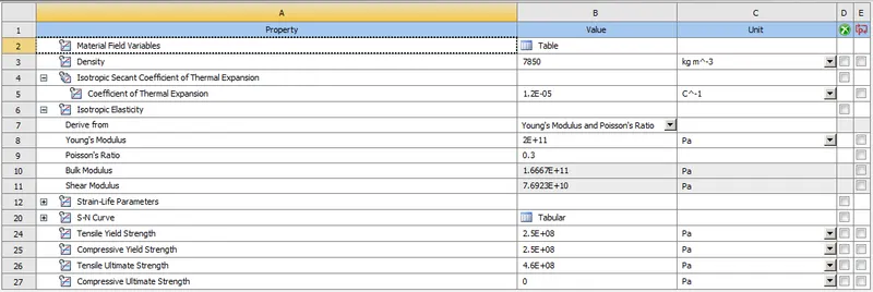
5. Material Properties:

5.1. For Workpiece: Copper Alloy NL.

                   

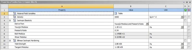
5.2. For Wheel: Structural Steel.

                   

6. PROCEDURE:

6.1. Import model in ANSYS Workbench.

6.2. Assign material properties.

6.3. Open the mechanical module, where we going to perform analysis.

6.4. Meshed the model with desired element size.

6.5. Now after meshing, From Project Tree, select "Connections" and create "Contact".

• Contacts:

1. Contact Type = Frictional 
2. Frictional Coeff. = 0.2
3. Behaviour = Program Controlled
4. formulation = Augmented Lagrange
5. Normal Stiffness Factor = 0.1
6. Interface treatment = Add Offset, Ramped Effects.

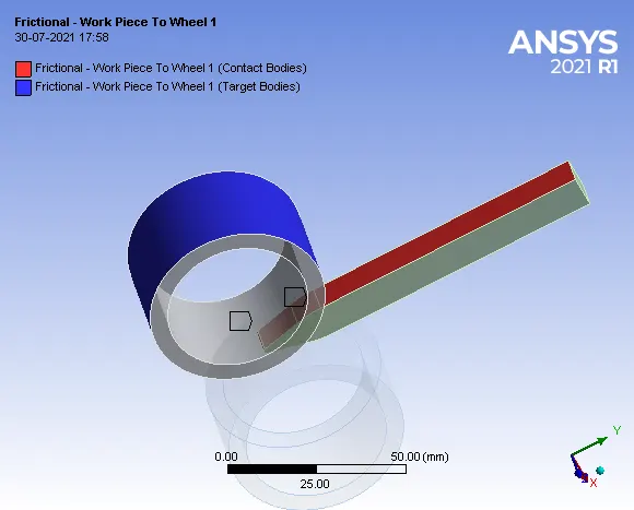
• The first contact between wheel 1 and one face of workpiece.

1. Contact Body = Workpiece
2. Target Body = Wheel 1

                                                                             

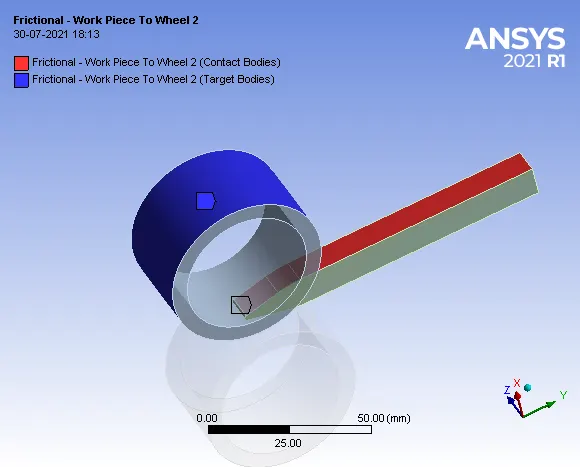
• The second contact between wheel 2 and one face of the workpiece.

1. Contact Body = Workpiece
2. Target Body = Wheel 2

                                                                             

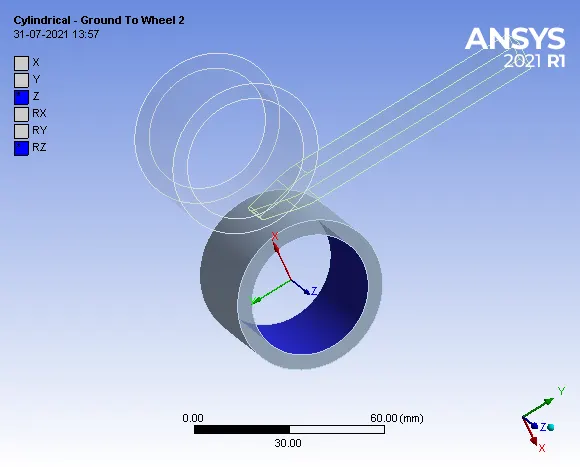
6.6. After defining proper contacts, Now define some joints for the wheel.

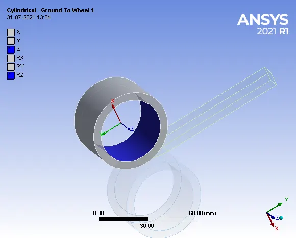
1. Connection Type = Body-ground.
2. Type = Cylindrical.

(A). Cylindrical- Ground to Wheel 1:

                                                                             

(B). Cylindrical- Ground to Wheel 2:

                                                                             

6.7. BOUNDARY CONDITIONS:

Now let's define the Boundary condition.

• Here we are going to look at stress, Strain and Deformation developed in the workpiece during the rolling operation.
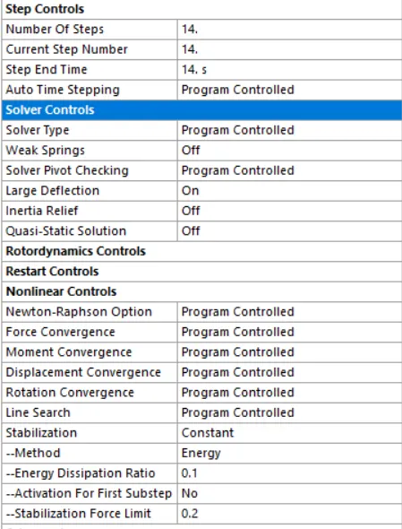
• In the analysis setting 

1. A number of Steps = 14.
2. Solver type = Program Controlled.
3. Turn ON Large deflection.
4. In Non-Linear controls:-

• Stabilization = Constant
• Method = Energy
• Energy Disipitation Ratio = 0.1

                                                                                                       

• Other boundary conditions are given below:

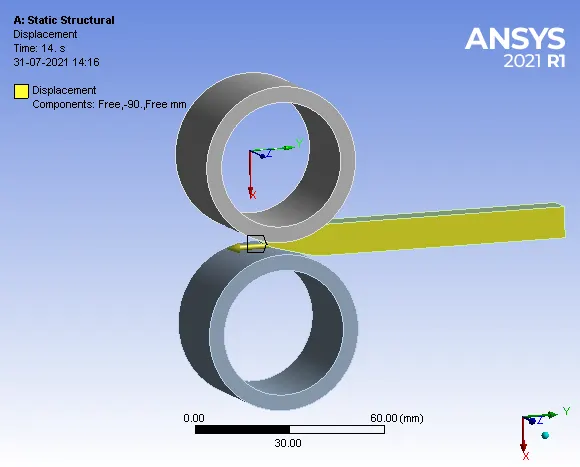
     1. Displacement of Workpiece In Y-Direction.

                                                                              

                                                                             

         2. Rotation of both Wheel, one is clockwise and the second is anti-clockwise.

                                                                              

                                                                             

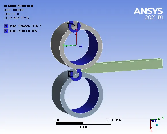
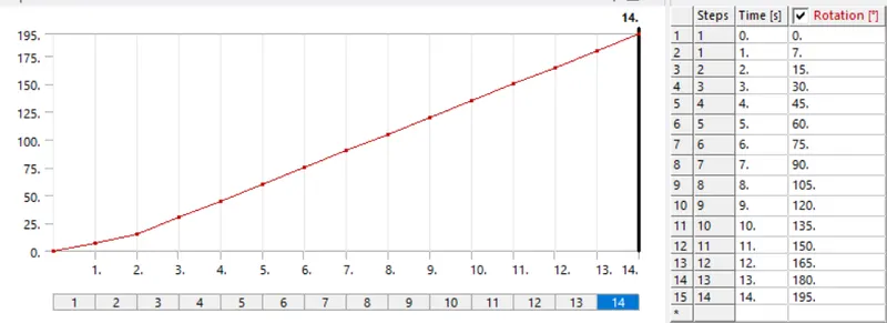
The displacement applied to the workpiece is such that it should displace by 90 mm. To pull in the workpiece for rolling operation, one of the wheels has to rotate clockwise and the other wheel has to rotate in the anti-clockwise direction. The rotation angle is specified from 0⁰ to 195⁰.

6.8. SOLUTION:

        After giving proper Boundary conditions, create a solution for the output result.

• Equivalent stress for the whole setup
• Equivalent Plastic strain for the workpiece
• Directional Deformation in the Z-axis for the workpiece
• Prove that the workpiece has been displaced by 90mm.

7. RESULT AND DISCUSSIONS:

7.1 Equivalent stress for the whole setup:

                                                                               

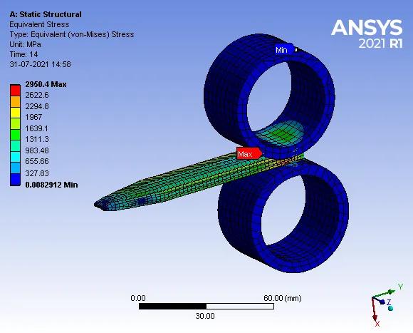
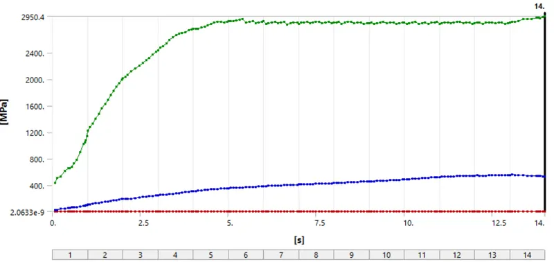
                                                                                                          Maximum Stress = 2950.4 MPa

• Stress Contours:

                                                             

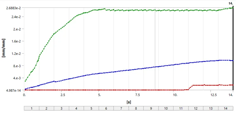
2. Equivalent Plastic strain for the workpiece:

                                                                                 

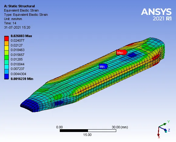
                                                                                                   Maximum Strain = 0.026883 mm/mm

• Strain Contours:

                                                             

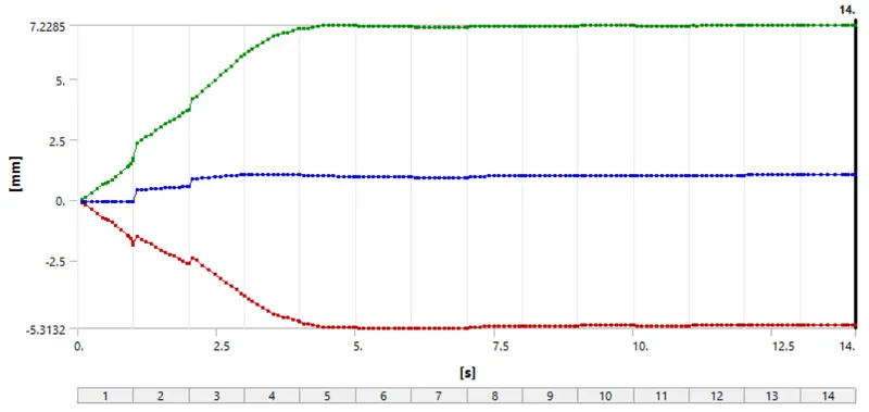
3. Directional Deformation in the Z-axis for the workpiece:

                                                                                 

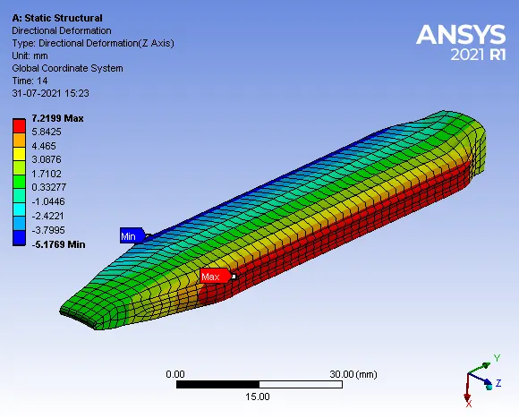
                                                                                                          Maximum Deformation = 7.2199 mm

• Deformation Contours:

                                                             

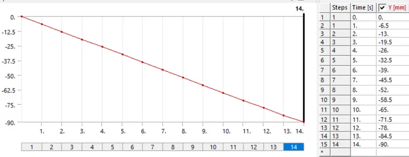
4. Directional Deformation in the Y-axis for the workpiece to show that it has displaced by 90mm.

                                                                                

                                                                       

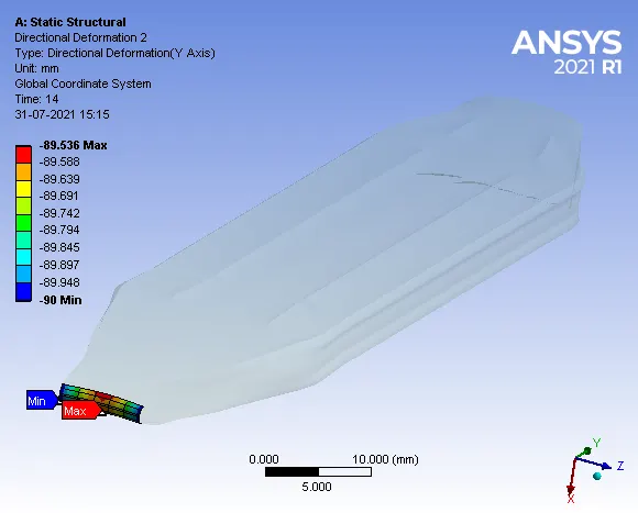
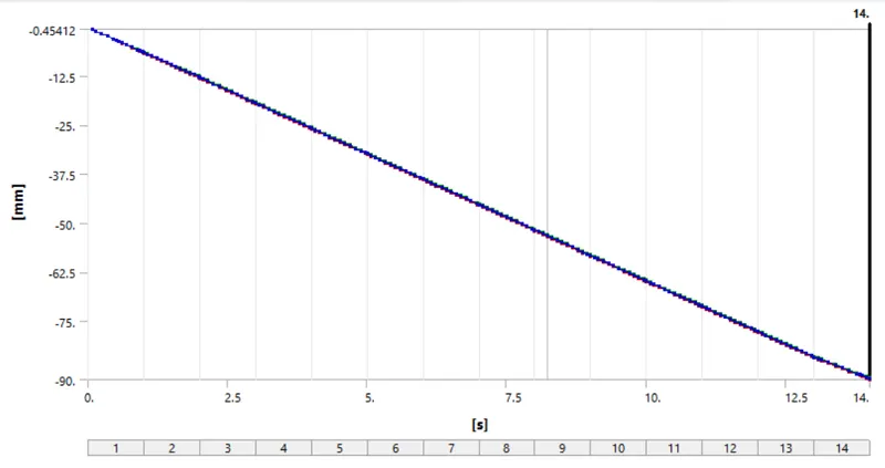
From the plot, it is observed that initially at time 0 s the workpiece was at 0.45412 mm in the negative Y-axis but at the end of the rolling operation i.e., at time 14 s, the workpiece is displaced to 90 mm in negative Y-axis. Hence, it is proved that the workpiece has been displaced by 90 mm.

                                                                                                                                                                                                                                                                                 

8. CONCLUSION

1. The given model was opened in Spaceclaim and the length of the workpiece was increased by 60 mm and its width was decreased by 8 mm on both sides.
2. The simulation of the rolling operation on a workpiece made of copper was made to run for 14steps successfully.
3. The Equivalent stress for the whole setup is 2950.4 MPa.
4. The Equivalent Plastic strain for the workpiece is 0.026883 mm/mm.
5. The Directional Deformation in the Z-axis for the workpiece is 7.2199 mm.
6. The Directional Deformation in the Y-axis for the edge of the workpiece is 90 mm. Hence, it is proved that the workpiece has been displaced by 90mm.