Week -4 : Optimisation of Stalagmite function
AIM : Optimisation of stalagmite function using genetic algorithm and obtaining the global maxima value of co-ordinates.
- Explaining about theory & Syntax of 'ga'.
- Finally , explaining about the three cases of genetic algorithm and F-maximum with no.of iteration.
GLOBAL EQUATIONS :
-
function:f
f(x,y)=f1,xf2,x f1,yf2,y
f1,x=[sin(5.1πx+0.6)]6
f1,y=[sin(5.1πy+0.6)]6
f2,x=exp[-4ln(2)(x-0.0667)2/0.64]
f2,y=exp[-4ln(2)(y-0.0667)2/0.64]
To find the global maxima of the function:F=-f
-ve sign because we have to find the function maximum.
- The above equation is a formulae which is created as a function and used to find the maximum value of genetic algorithm for stalagmite model.
OBJECTIVES:
- Main objective is knowing about the genetic algorithm which is used to obtain the maximum value.
- GENETIC ALGORITHM : The genetic algorithm is a method for solving both constrained and unconstrained optimization problems that is based on natural selection, the process that drives biological evolution. The genetic algorithm repeatedly modifies a population of individual solutions.
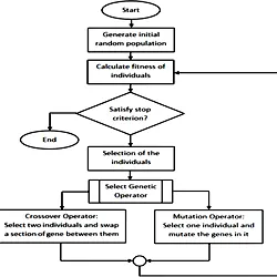
- HOW DOES IT WORKS :
- Initial population : Algorithm begins by creating a random initial population. For example, if you believe that the minimal point for Rastrigin's function is near the point
[0 0], you could set Initial population Range to be[-1;1]. - Parent: Group of individuals in the current population.
- Creating the Next Geneartion:At each step, the genetic algorithm uses the current population to create the children that make up the next generation. The algorithm selects a group of individuals in the current population, called parents, who contribute their genes—the entries of their vectors—to their children. The algorithm usually selects individuals that have better fitness values as parents.
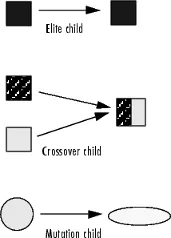
The genetic algorithm creates three types of children for the next generation:
-
Eliteare the individuals in the current generation with the best fitness values. These individuals automatically survive to the next generation.
-
Crossover are created by combining the vectors of a pair of parents.
-
Mutation children are created by introducing random changes, or mutations, to a single parent.
The following schematic diagram illustrates the three types of children.
- Fitness Function-The fitness function is used to determine the individual's fitness level in the population. It means the ability of an individual to compete with other individuals. In every iteration, individuals are evaluated based on their fitness function.
-
Crossover Children
The algorithm creates crossover children by combining pairs of parents in the current population. At each coordinate of the child vector, the default crossover function randomly selects an entry, or gene, at the same coordinate from one of the two parents and assigns it to the child. For problems with linear constraints, the default crossover function creates the child as a random weighted average of the parents.
Mutation Children
The algorithm creates mutation children by randomly changing the genes of individual parents. By default, for unconstrained problems the algorithm adds a random vector from a Gaussian distribution to the parent. For bounded or linearly constrained problems, the child remains feasible.
-
Plots of Later Generations:
The following figure shows the populations at iterations 60, 80, 95, and 100.
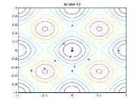
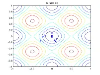
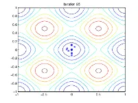
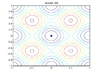
NOTE: As the number of generations increases, the individuals in the population get closer together and approach the minimum point
[0 0].Stopping Conditions for the Algorithm
The genetic algorithm uses the following options to determine when to stop. See the default values for each option by running opts=optimoptions('ga).
-
Maxmium generations — The algorithm stops when the number of generations reaches
MaxGenerations. -
Maxtime — The algorithm stops after running for an amount of time in seconds equal to
MaxTime. -
Fitness limit — The algorithm stops when the value of the fitness function for the best point in the current population is less than or equal to fitness limit .
SYNTAX of Genetic Algorithm:
For more information , please check with this link provided below,
https://in.mathworks.com/help/gads/how-the-genetic-algorithm-works.html
BODY OF CONTENT :
-
close all clear all clc %Defining the space x = linspace(0,1,150); y = linspace(0,1,150); %Creating the 2D Dimensional mesh [xx,yy] = meshgrid(x,y); for i = 1:length(xx) for j = 1:length(yy) input_vector(1) = xx(i,j); input_vector(2) = yy(i,j); f(i,j) = stalagmite(input_vector); end end surfc(xx,yy,-f); xlabel('x'); ylabel('y'); shading interp [inputs,fval] = ga(@stalagmite,2) num_cases = 50; tic %study 1 statistical behaviour for i=1:num_cases [inputs,fopt(i)]=ga(@stalagmite,2); xopt(i)=inputs(1); yopt(i)=inputs(2); end study1_time=toc %plotting_graph figure(1) subplot(2,1,1) hold on surfc(xx,yy,-f) shading interp plot3(xopt,yopt,-fopt,'Marker','o','MarkerSize',5,'MarkerFaceColor','r') title('Unbounded inputs') subplot(2,1,2) plot(-fopt) xlabel('iterations') ylabel('function_minimum') tic %study 2 statistical behaviour with upper and lower bounds for i=1:num_cases [inputs,fopt(i)]=ga(@stalagmite,2,[],[],[],[],[0,0],[1,1]); xopt(i)=inputs(1); yopt(i)=inputs(2); end study2_time=toc %plotting_graph figure(2) subplot(2,1,1) hold on surfc(xx,yy,-f) shading interp plot3(xopt,yopt,-fopt,'Marker','o','MarkerSize',5,'MarkerFaceColor','r') title('Bounded inputs') subplot(2,1,2) plot(-fopt) xlabel('iterations') ylabel('function_minimum') %study 3 Increasing ga iterations options = optimoptions('ga'); options = optimoptions(options,'populationsize',170); tic for i=1:num_cases [inputs,fopt(i)]=ga(@stalagmite,2,[],[],[],[],[0,0],[1,1],[],[],options); xopt(i)=inputs(1); yopt(i)=inputs(2); end study3_time=toc %plotting_graph figure(3) subplot(2,1,1) hold on surfc(xx,yy,-f) shading interp plot3(xopt,yopt,-fopt,'Marker','o','MarkerSize',5,'MarkerFaceColor','r') title('Bounded inputs with increase in Population') subplot(2,1,2) plot(-fopt) xlabel('iterations') ylabel('function_minimum') -
STALAGMITE_FUNCTION :
function f = stalagmite(input_vector)


x = input_vector(1);
y = input_vector(2);

f1x = [sin(5.1*pi*x+0.5)]^6;
f1y = [sin(5.1*pi*y+0.5)]^6;

A = (x-0.0667)^2/0.64;
B = (y-0.0667)^2/0.64;

f2x = exp(-4*log(2)*A);
f2y = exp(-4*log(2)*B);

f = -(f1x*f2x*f1y*f2y);

end
COMMENTS FOR THE CODE :
1.Starting with Clear all,close all and clc i.e it mean to clearing the data and closing
  all the figure windows and clearing the data in command window.
2.Defining the space upto which limit the gentic algorithm should generate the population.
3.Creating the 2D mesh by using the 'MESHGRID' command and using the for loop to evaluate
  the stalagmite function again and again.
4.A stalagmite function generally refers to the function with which we are generating
  values over a stalagmite kind of surface for finding out the local and global maxima and
  minima of that particularly given function

  A stalagmite appears like an inverted stalactite, rising from the floor of a cavern.
5.We will be writing a code for stalagmite function to evaluate the globsl maxima value
  and local minima value.
6.X-label means representing the any label to the x-axis.
  Y-label means representing the any label to the y-axis.
7.Next, we will be evaluating the all cases related to gentic algorithm of various
  conditions.
8.As a sample , we will be assuming the no.of iteration.
9.For the first case of statistical behaviour,we will be using x = ga(fun,nvars) finds a
  local unconstrained minimum, x, to the objective function, fun. nvars is the dimension
  (number of design variables) of fun.
  In this case we can use sub-plots to get a multiple plots in a one figure window.
  So,here we can get a plot related to surf(xx,yy,-f)and one more plot related to the
  iterations Vs function_maximum.
  Here.we can see unbounded inputs exceeding the range .
  Note : -f signs that to optimize the global maximum value.

10.For the second case of statistical behaviour with upper and lower bounds,we will be
   using the x = ga(fun,nvars,A,b,Aeq,beq,lb,ub) defines a set of lower and upper bounds
   on the design variables, x, so that a solution is found in the range lb ≤ x ≤ ub. (Set
   Aeq=[] and beq=[] if no linear equalities exist.)
   Here , we can see the plot with bounded inputs within the range.

11.For the third case of Increasing the ga iterations.x =
   ga(fun,nvars,A,b,Aeq,beq,lb,ub,nonlcon,intcon) or x =
   ga(fun,nvars,A,b,Aeq,beq,lb,ub,nonlcon,intcon,options) requires that the variables
   listed in intcon take integer values.

   And,

   options = optimoptions(SolverName) returns a set of default options for the SolverName
   solver.

   options = optimoptions(SolverName,Name,Value) returns options with specified
   parameters set using one or more name-value pair arguments.

   Here, we can get bounded inputs with increase in population.
ERRORS:
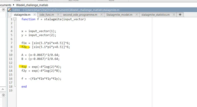
Solution :
In the line8 and line13,
i have done a mistake regarding formulae, it should coded as 'f1y' in line8 and 'f2x' in line13.
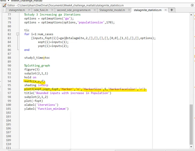
Solution:
In Line94 & Line96,
i have made a mistake regarding the surfc plot and plot3,in line94 it should be coded as surfc(xx,yy,-f) and
in line96 it should be coded as plot3(xopt,yopt,-fopt,.....).
CONCLUSIONS :
Here , please go through the solution or plots which i have generated by using the above mentioned code.
https://drive.google.com/file/d/1fyt87c1tG1gfKxL4ikjQeGgmGx9aWDKf/view?usp=sharinghttps://drive.google.com/file/d/1fyt87c1tG1gfKxL4ikjQeGgmGx9aWDKf/view?usp=sharinghttps://drive.google.com/file/d/1ubqZcMKhmYwN4UZPxZg2Co9cwhJQIywI/view?usp=sharing
THANK YOU !!