Week 3 - Solving second order ODEs
%A PROGRAMME TO SIMULATE THE MOMENTUM OF THE PENDULUM BY USING SECOND_ODE :

%Second_odrer_ode_programm
close all
clear all
clc

%inputs
b = 0.05;
m = 1;
l = 1;
g = 9.81;

%input_conditions
theta_0 = [0;3];   %intial displacement and intial velocity

%time_points
t_span = linspace(0,20,500);

%solve_ode
[t,results] = ode45(@(t,theta) ode_func(t,theta,b,m,g,l),t_span,theta_0);

plot(t,results(:,1))
hold on
plot(t,results(:,2))
xlabel('time')
ylabel('plot')

%Animation_of_pendulum
displacement = results(:,1);
ct = 1;
for i = 1 : length(displacement)
    angle = displacement(i);
    x0 = 0;
    y0 = 0;
    x1 = 1*sin(angle);
    y1 = -1*cos(angle);

    figure(2)
    plot([-1.1 1.1],[0 0],LineWidth=3);
    hold on
    plot([x0 x1],[y0 y1],'linewidth',3)
    title('SIMPLE PENDULUM')

    plot(x1,y1,'o','markers',20,'markerfacecolor',[1 1 0]);
    hold off
    grid on
    axis([-1.5 1.5 -1 1])
    pause(0.01)
    M(ct) = getframe(gcf);
    ct=ct+1 ;
end

movie(M)
videofile = VideoWriter('Simple_pendulum.avi','Uncompressed AVI');
open(videofile)
writeVideo(videofile,M)
close(videofile)
ODE_FUNCTION_CODE :
%A PROGRAMME DEFINES THE SECOND_ODE FUNCTION :

function[dtheta_dt] = ode_func(t,theta,b,m,g,l)

theta1 = theta(1);
theta2 = theta(2);
dtheta1_dt = theta2;
dtheta2_dt = -(b/m)*theta2-(g/l)*sin(theta1);
dtheta_dt = [dtheta1_dt;dtheta2_dt]
end
COMMENTS :
EXPLANATION OF CODE :
- We have our aim to plot the momentum of pendulum by using the initial condition with the
second oder differential equation . - in the above of the code we have assumed the initial condition which are related to the simple pendulum .
- Next , the given conditions were angular displacement and velocity , these are solution vectors which were stored in array .
- we have to simulate the pendulum between the given timespan,so to create that count we will be using the linspace command .
- [t,results] = ode45(@(t,theta) ode_func(t,theta,b,m,g,l),t_span,theta_0);
- The above line represents solving ode ,so here we will be using the(t,theta) as dependent variables and using the function followed by the initial conditions .
- Actually ODE is a in-built solver .
- Next , the results will be defined which were stored in array by using that we can get a plot as below :
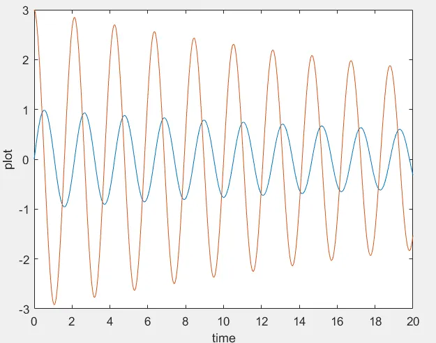
- But , we need to get a simulated plot of pendulum , for that the rest of the code belongs to it .
- To simulate the motion , we need store the data in for loop and we need to define the position of
co-ordinates . - After , we ne ed to use hold option so the previous plot will be override.
- For the next plot we need to use fresh window i.e figure (2) .
- Finally , we need to plot these values and give the label names & we will be using the counter so the for loop will be executed for multiple times .
- The counter value will be stored in the array and that stored data will be used to create a movie file to get a smooth simulation .
ODE_FUNCTION EXPLANATION :
- we have one more code which has mentioned above that means in solving the ODE we have been used the ode_func with the inputs .
- We willl create a programme regarding the function in the same directary and that code will be called to the main code , so the size of the code will be reduced and code looks good .
- In the ode function code , we will be creating the programme for the second order differential equations .
DETAILED_REPORT :
https://skill-lync.com/myprojects
SIMULATION OF PENDULUM :
https://drive.google.com/file/d/1I-EfkJWeAA6DIli52Iy_HQfnHDAvm_Q3/view?usp=sharing
SECOND_ODE_PLOT:
https://drive.google.com/file/d/1Ovx4uc3ILw7UJ73on_03zhoTwY9lcHn7/view?usp=sharing