Week-4 : CURVE FITTING

Curve fitting : Curve fitting is a process of constructing of a curve which posses the closest proximity to the real series of data . By curve fitting , we can mathematically construct the functional relationship between the data set and parameter values .

METHODS TO GET BEST FIT :

• THE SUM OF SQUARES DUE TO ERRORS .
• R-SQUARE .
• ADJUSTED R - SQUARE .
• ROOT MEAN SQUARED ERROR .

AIM :

• Write code to fit a linear and cubic polynomial for the Cp data.
• Plot the linear and cubic fit curves along with the raw data points.
• Write a code to show splitwise method.
• Measure the fitness characteristics for both the curves .

GOVERNING EQUATIONS :

• R_SQUARE :

The quantity that measures how successful the fit is in variation of data and it refers that square of sum o fthe square of correction between the responsed values to the predicted response values .

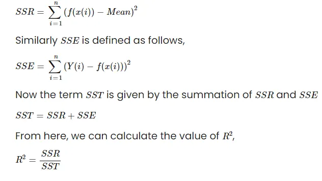
• Adjusted R_square: It is variation function r_square which neglect the independent values of r_square .

So , we will be finding the both values of adjusted R_Square and R_Square .

By that we can calculate the goodness of fit for curve .

formulae :

`R^2 adj = 1- [(1-R^2)(n-1)//(n-k-1)]`

NOTE : R_square = 1 (best fit) .

R_square = 0 (bad fit) .

OBJECTIVES OF PROJECT :

• Here , the main objective is to relate the curve of existing dataset and predicted dataset .
• From the below image , we can see the interaction between the two curve . So , our aim is to define and verify the goodness between them .

BODY OF PROGRAMME :

close all
clear all
clc

% Data_creation
cp_data = load('data');
Temperature = cp_data(:,1);
cp = cp_data(:,2);

% NOTE : Specific_heat is a function of Temperature.

co_efficients = polyfit(Temperature,cp,3);
predicted_cp = polyval(co_efficients,Temperature);

%compare
plot(Temperature,cp,LineWidth=3,Color='r')
hold on
plot(Temperature,predicted_cp,'Linewidth',3,'Color','b')
ylabel('cp')
xlabel('temperature')
legend('Orginal data','curve fit')

%Calculation_for_best_fit_curve
mean = sum(cp)/3200;
for i = 1:length(Temperature)
    x(i) = (predicted_cp(i)-cp(i))^2;
end

for j = 1:length(cp)
    y(j) = (predicted_cp(j)-mean)^2;
end


SSE = sum(x); 
SSR = sum(y);
SST = SSE+SSR;
R_SQUARE = SSR/SST

n = 3200;
k = 0;

P = (1-R_SQUARE)*(n-1);
Q = (n-k-1);
Adj_Rsquare = 1-(P/Q)
RMSE = (SST/n)^0.5

COMMENTS :

1 . Firstly , we have to store our data in the respective directory and redierecting that 
    file into the code which consists of two columns i.e Temperature , Specific Heat.

2 . Next , our aim is to find the cubic fit curve so we can obtain the co-efficients of 
    cubic polynomial by polyfit and to obtain that polynomial co-efficients by polyval 
    command .

3 . So , we wiil be storing the polyval in tha variable of predicted cp.

4 . Then , we will be interacting the curves of linear and cubic fit .

5 . the plot will be attached below .

https://drive.google.com/file/d/1JLeiKgh6A5mTiG8y1yO4fli9RzLkt1OR/view?usp=sharing

6 . Calculation of best fit curve - here we will be using the four methods for to rectify the goodness of the curve .
  
  we will be starting with the R_square :
  
  1. In this related topic we will find the values for the SSR and SSE .
  2. Finally we can obtain the R_square values and Adjustable R_square .
  3. So, if the values which are obtain near to 1 or equal to 1 is the best fit curve .
  
Note : please refer the image below for the calculated solution .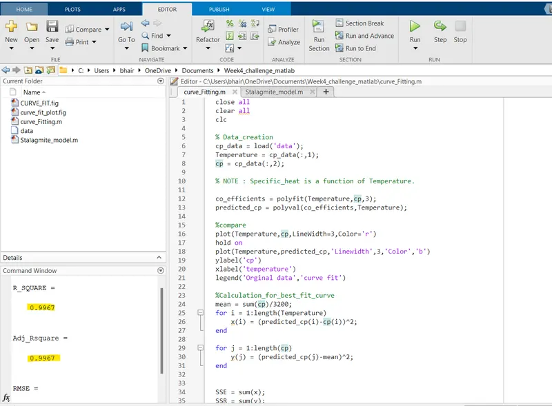

ERROR :

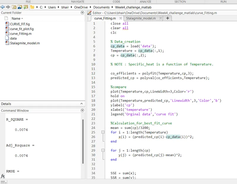
Line 26 - We have the unrecognised variable i.e cp_data instead of that we will correct as cp.

Because , the cp_data both temperature and specific .

CONCLUSION :

https://drive.google.com/file/d/1JLeiKgh6A5mTiG8y1yO4fli9RzLkt1OR/view?usp=sharing

https://drive.google.com/file/d/1ys4OsMirthpu6nA9gHoZQEXd2vSybBLJ/view?usp=sharing

Thank you !!