AIR_STANDARD_OTTO_CYCLE
DETAIL REPORT ON AIR_STANDARD_OTTO_CYCLE
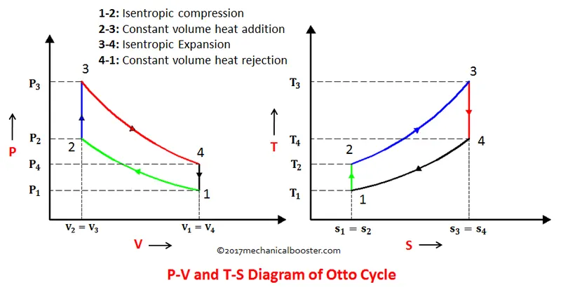
- Otto_cycle : An Otto cycle is an idealized thermodynamic cycle that describes the functioning of a spark ignition piston engine which is the thermodynamic cycle .
- Process of otto cycle : 1 . ISENTROPIC COMPRESSION .
2 . CONSTANT VOLUME HEAT ADDITIION .
3 . ISENTROPIC EXPANSION .
4 . CONSTANT VOLUME HEAT REJECTION .
- AIM :
- Creating the code to plot the pressue-volume diagram of otto cycle .
- Calculating the thermal efficiency of the air standard otto cycle .
- GOVERNING EQUATIONS :
- Ideal gas equation :

2. Isentropic Equation :
P = constant / Vκ
3. The above equations were used at different state of points i.e ISENTROPIC CONDITION & CONSTANT VOLUME PROCESS .
- OBJECTIVE OF THE PROJECT :
- Creating the code to plot the pressue-volume diagram of otto cycle & Calculating the thermal efficiency of the air standard otto cycle .
-
BODY OF THE CONTENT :
* FIRST PROGRAMME
close all

clear all

clc

%input

gamma = 1.4 ;

%state_vriables

p1 = 101325;

t1 = 500;

t3 = 2500;

%engine_geometric parameters

bore = 0.1;

stroke = 0.1;

cr = 12;

con_rod = 0.15;

%swept vol, clearance vol

v_swept = (pi/4)*bore^2*stroke;

v_clearance = v_swept/(cr-1);

v1 = v_swept + v_clearance;

v2 = v_clearance;

%condition_at_state_point_2

%p2v2^gamma = p1v1^gamma

%p2 = p1*(v1/v2)^gamma

p2 = p1*cr^gamma;

%p1v1/t1 = p2v2/t2

t2 = p2*v2*t1 / (p1*v1);

%condition_at_state_point_3_using_ideal_gas_equation

v3 = v2;

%pv=t; p2v2/t2 = p3v3/t3

p3 = p2*t3/t2

%condition at state point 4

v4 = v1;

%p3v3^gamma = p4v4^gamma

p4 = p3*(v3/v4)^gamma

figure(1)

hold on

plot(v1,p1,'*','color','g')

plot(v2,p2,'*','color','g')

plot(v3,p3,'*','color','g')

plot(v4,p4,'*','color','g')


OUTPUT :
https://drive.google.com/file/d/1DUp5hn1uzV7EDa9u2QwdvAwWaWh45tJg/view?usp=sharing
* SECOND PROGRAMME
function [V] = engine_kinematics(bore,stroke,cr,con_rod,Start_crank,end_crank)

%bore = 0.1;

%stroke = 0.1;

%cr = 12;

%con_rod = 0.15;

a = stroke/2;

R = con_rod/a;    %ratio of con rod to the crank pin radius

v_swept = (pi/4)*bore^2*stroke;

v_clearance = v_swept/(cr-1);

theta = linspace(Start_crank,end_crank,720);

term_1 = 0.5*(cr-1);

term_2 = R+1-cosd(theta);

term_3 = (R^2-sind(theta).^2).^0.5;

V = (1+term_1*(term_2-term_3))*v_clearance;

end


OUTPUT:
https://drive.google.com/file/d/1DrT1GtR5lSsz_BbR7w8j8MFd9xsfTi3E/view?usp=sharing
* THIRD PROGRAMME :
%Engine_kinematics_final_code

close all

clear all

clc

%input

gamma = 1.4 ;

%state_vriables

p1 = 101325;

t1 = 500;

t3 = 2500;

%engine_geometric parameters

bore = 0.1;

stroke = 0.1;

cr = 12;

con_rod = 0.15;

%swept vol, clearance vol

v_swept = (pi/4)*bore^2*stroke;

v_clearance = v_swept/(cr-1);

v1 = v_swept + v_clearance;

v2 = v_clearance;

%condition_at_state_point_2

%p2v2^gamma = p1v1^gamma

%p2 = p1*(v1/v2)^gamma

p2 = p1*cr^gamma;

constant_c = p1*v1^gamma

v_compression = engine_kinematics(bore,stroke,cr,con_rod,180,0)

p_compression = constant_c./(v_compression.^gamma)

%p1v1/t1 = p2v2/t

t2 = p2*v2*t1 / (p1*v1);

%condition_at_state_point_3_using_ideal_gas_equation

v3 = v2;

%pv=t; p2v2/t2 = p3v3/t3

p3 = p2*t3/t2

constant_c = p3*v3^gamma

v_expansion = engine_kinematics(bore,stroke,cr,con_rod,0,180)

p_expansion = constant_c./(v_expansion.^gamma)

%condition at state point 4

v4 = v1;

%p3v3^gamma = p4v4^gamma

p4 = p3*(v3/v4)^gamma

figure(1)

hold on

plot(v1,p1,'*','color','g')

plot(v_compression,p_compression)

plot(v2,p2,'*','color','g')

plot(v3,p3,'*','color','g')

plot(v_expansion,p_expansion)

plot(v4,p4,'*','color','g')

OUTPUT :
https://drive.google.com/file/d/1fgF1xpPujSyVLIw-dOJpf2RNVhXyRaaD/view?usp=sharing- EXPLANATION OF ABOVE MENTIONED PROGRAMMES :
COMMENTS :

1. The first code describes about the plotting of the volume-pressure diagram :

   Body of the programme describes the inputs of the engine geometry factors which were
   used to define engine volume kinematics.

   Defining the global equations i.e the isentropic equations and constant volume
   expressions.

   So,the state of variables which atre pressure , temperature and volume were defined.
   Finally , by using the state variables the plot is defined and drive link is attached
   at the end of the code.

   Finally , we can define only the points of the various states in the plot but it is
   not efficient .


2. The Second code programme describes which is more efficient than the first one.


    where the one more equation comes into picture which is defined from the engine
    kinematics to solve the volume .

    So , we define the volume by using the angles which were required in the combustion
    process in the engine i.e TDC to BDC (0 to 180)...

    Here , using the linkspace command we can get count of the varies values of angles.

    But , we will be using the function command instead of pasting the second code in
    the first one .

    where the function inputs will be defined and we ca called in the main code i.e first
    code.

    but by using the second body of code , we can get a output and drive link is
    provided .

3. The third code programme describes which is the efficient one which can describes the
    complete PV diagram of the air standard cycle .


   in this code we will be caaling the function inputs in to this code and make the code
   easy to derive the plot ,

   At , the compression and expansion the function has been called so that by using those
   values the plot can be defined at the compression and expansion .

  NOTE : THE FUCTION INPUT FILE SHOULD EXIST IN THE SAME FOLDER TO CALL THE FUNCTION INTO
  THE ANOTHER CODE .
  THE FUNCTION NAME WHICH IS CONSIDERED IN THE CODE , MUST BE THE FILE NAME .
- ERRORS :
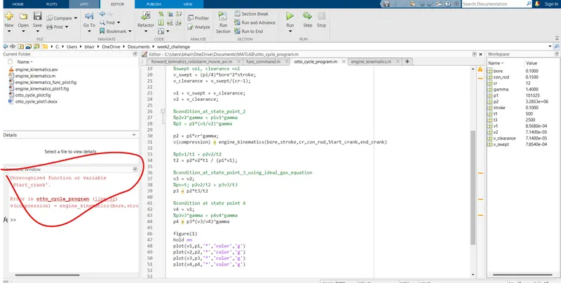
ANSWER : V(COMPRESSION) = ENGINE_KINEMATICS(,,,,,,,,,,,0,180)
in the function inputs , the variables are represented but not recognised with certain value .
so while calling the function , we need to define the values .
- CONCLUSION :
THE VARIOUS PLOTS WHICH WILL BE MENTIONED BELOW AGAIN :
https://drive.google.com/file/d/1DUp5hn1uzV7EDa9u2QwdvAwWaWh45tJg/view?usp=sharing
https://drive.google.com/file/d/1DrT1GtR5lSsz_BbR7w8j8MFd9xsfTi3E/view?usp=sharing
https://drive.google.com/file/d/1fgF1xpPujSyVLIw-dOJpf2RNVhXyRaaD/view?usp=sharing
NOTE : THERMAL EFFICIENCY OUTPUT LINK MENTIONED BELOW :
https://drive.google.com/file/d/1xxfPpPne9FgJzciQ0dXOA_UJvs42dQkq/view?usp=sharing
BEST REGARDS,
SRINIVAS BHAIRI .