Week 4 - Genetic Algorithm
Genetic Algorithm By Using Of MATLAB
Aim Of Project:-
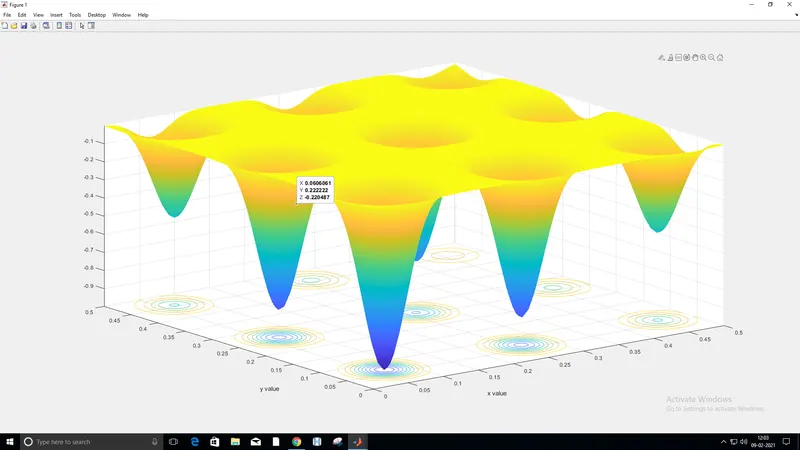
Write a code in MATLAB to optimise the stalagmite function and find the global maxima of the function and also explain the concept
of genetic algorithm. Use of syntax 'ga'.
Introduction :-
Genetic algorithm was born by the "John Holland",according to this process transfer the best output for next genration .
In this case we got multiple solution but we target only optimum solution(best solution).
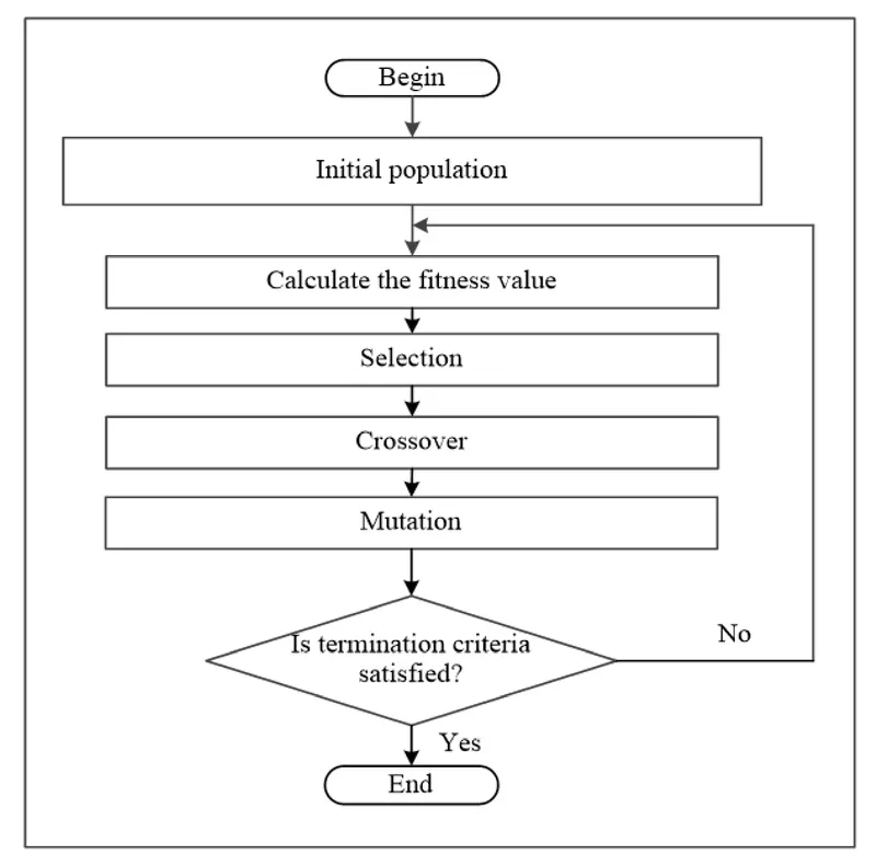
All are the depends upon fitness value which can be help to finding the best result. Genetic algorithm is a method for solving both constrained and unconstrained optimization problems based on a natural selection process that mimics biological evolution.
The algorithm repeatedly modifies a population of individual solutions. At each step, the genetic algorithm randomly selects individuals from the current population and uses them as parents to produce the children for the next generation.
Over successive generations, the population evolves toward an optimal solution.
Application Of GA:-
-
Scheduling applications − GAs are used to solve various scheduling problems as well, particularly the time tabling problem.
-
Machine Learning − as already discussed, genetics based machine learning (GBML) is a niche area in machine learning.
-
Robot Trajectory Generation − GAs have been used to plan the path which a robot arm takes by moving from one point to another.
-
Parametric Design of Aircraft − GAs have been used to design aircrafts by varying the parameters and evolving better solutions.
-
DNA Analysis − GAs have been used to determine the structure of DNA using spectrometric data about the sample.
-
Multimodal Optimization − GAs are obviously very good approaches for multimodal optimization in which we have to find multiple optimum solutions.
-
Traveling salesman problem and its applications − GAs have been used to solve the TSP, which is a well-known combinatorial problem using novel crossover and packing strategies.
for more inf.
https://www.analyticsvidhya.com/blog/2017/07/introduction-to-genetic-algorithm/
Referance:-
https://www.youtube.com/watch?v=96-u9s6D16k
https://en.wikipedia.org/wiki/Genetic_algorithm
Input Function
f(x,y)= f1,x. f2,x. f1,y.f2,y
where
f1,x= [sin(5.1*pi*x+0.5)]^6
f1,y= [sin(5.1*pi*y+0.5)]^6
f2,x= exp[-((4ln(2)(x-0.0667)^2)/0.64)]
f2,y=exp[-((4ln(2)(y-0.0667)^2)/0.64)]
MATLAB Code:-
close all
clear all
clc
%define our search space
x= linspace(0,0.5,100);
y= linspace(0,0.5,100);
%creating 2D mesh array
[xx yy]= meshgrid(x,y);
% evaluating the staglamite function
for i= 1:length(xx);
for j= 1:length(yy);
input_vector(1)= xx(i,j);
input_vector(2)= yy(i,j);
f(i,j) = stalagmite(input_vector);
end
end
surfc(yy,xx,f);
xlabel('x value')
ylabel('y value')
shading interp
[x , fval]= ga(@stalagmite,2)
FUNCTION CODE:-
function [f]= get_stalagmite(input)
x= input(1);
y= input(2);
f1= (sin(5.1*pi*x+0.5))^6
f2= [sin(5.1*pi*y+0.5)]^6
f3 = exp((-4*log(2)*((x-0.0667).^2))./0.64)
f3 = exp((-4*log(2)*((y-0.0667).^2))./0.64)
f = -(f1*f2*f3*f4)
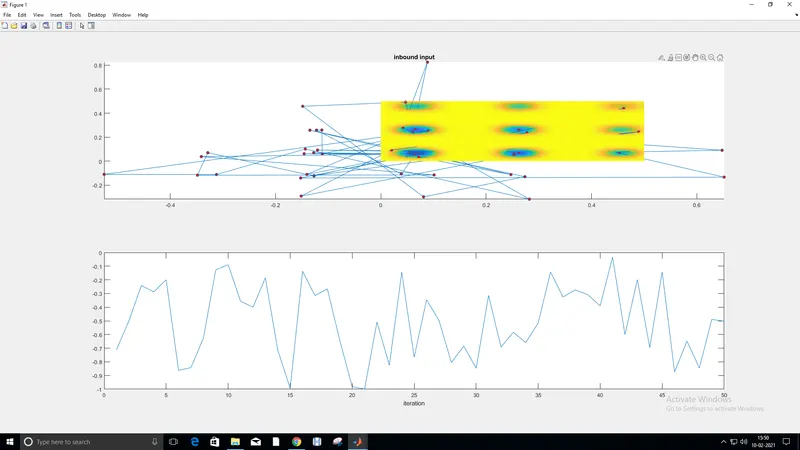
Unbounded Statastical Behvaiour
num_case= 50
% study 1 - statical behavior
for i= 1:num_case
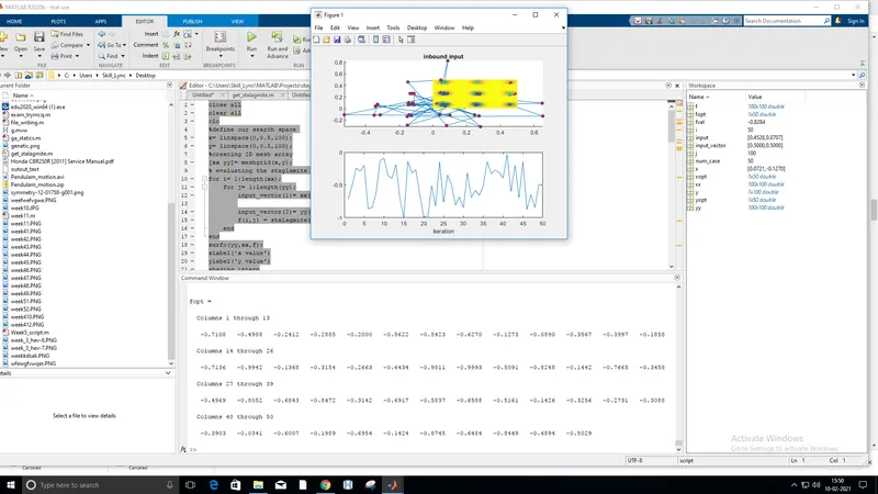
[input,fopt(i)]= ga(@stalagmite,2)
xopt(i)= input(1);
yopt(i)= input(2);
end
%study_time= toc
figure(1)
subplot(2,1,1);
hold on
surfc(xx,yy,f);
shading interp
plot3(xopt,yopt,fopt,'marker',
title('inbound input');
subplot(2,1,2);
plot(fopt);
xlabel('iteration')
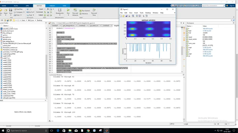
Output
STUDY 2ND
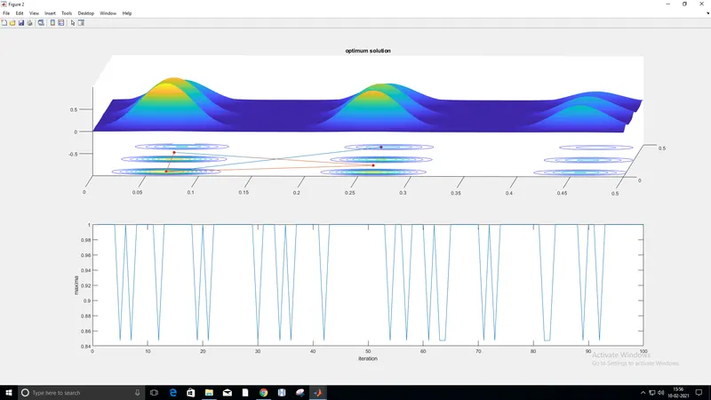
Bounded statastical Behvaiour
num_case = 100;
for i= 1:num_case
[input,fopt(i)]= ga(@stalagmite,2,[],[],[],[],[
xopt(i)= input(1);
yopt(i)= input(2);
end
%study_time2= toc
figure(2)
subplot(2,1,1);
hold on
surfc(xx,yy,-f);
shading interp
plot3(xopt,yopt,fopt,'marker',
title('inbound input');
subplot(2,1,2);
plot(-fopt);
xlabel('iteration')
Output
STUDY 3RD
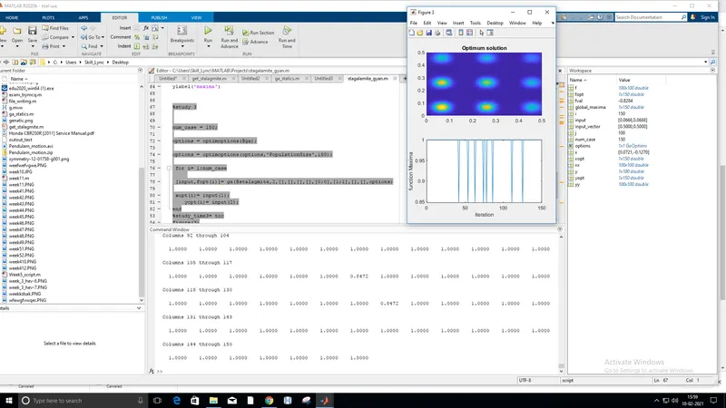
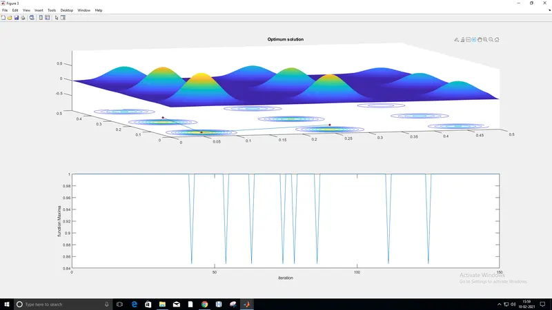
Modified Population Size Plot
num_case = 150;
options = optimoptions(@ga);
options = optimoptions(options,'
for i= 1:num_case
[input,fopt(i)]= ga(@stalagmite,2,[],[],[],[],[
xopt(i)= input(1);
yopt(i)= input(2);
end
%study_time3= toc
figure(3)
subplot(2,1,1);
hold on
surfc(xx,yy,-f);
shading interp
plot3(xopt,yopt,fopt,'marker',
title('Optimum solution');
subplot(2,1,2);
plot(-fopt);
xlabel('iteration')
ylabel('function Maxima')
global_maxima= -fopt
Output
Explanation Function Program:-
Function is declared first and then define the input vector define.
Then input the function and use negative sign in function because want the maxima.
Explanation of Main Program:-
- First use linspace to define x and y in 100 element b/w 0 to 0.5.
- Num_case to set for counter interation the value of 50.
- meshgrid use for convert of x and y in 2d.
- the loops involve to solve the GA for 2D mesh.
- stalagmite use for genration of maxima or minima.
- [input, fopt]= ga(fun, nvars)
where
input- show the value of x and y for least valure of function
fun- function optimization for case of stalagmite
nvars- variable which are ploted, in this case x and y is variable
toc - use for timer
In case of bounded
[input,fopt]= ga(fun, nvars,A,b,Aeq,beq,lb,ub)
input- show the value of x and y for least valure of function
fun- function optimization for case of stalagmite
nvars- variable which are ploted, in this case x and y is variable
A- Linear inequality Constraints: real matrix,if there are none, then[]
b-Linear inequality Constraints: real vector,if there are none, then[]
Aeq-Linear inequality Constraints: real matrix,if there are none, then[]
beq-Linear inequality Constraints: real vector,if there are none, then[]
lb- lower bounds
ub-upper bounds
The papulation size study
[input,fopt]= ga(fun, nvars,A,b,Aeq,beq,lb,ub,nonlcon,intcon,options)
[input,fopt]= ga(fun, nvars,A,b,Aeq,beq,lb,ub)
input- show the value of x and y for least valure of function
fun- function optimization for case of stalagmite
nvars- variable which are ploted, in this case x and y is variable
A- Linear inequality Constraints: real matrix,if there are none, then[]
b-Linear inequality Constraints: real vector,if there are none, then[]
Aeq-Linear inequality Constraints: real matrix,if there are none, then[]
beq-Linear inequality Constraints: real vector,if there are none, then[]
lb- lower bounds
ub-upper bounds
nonlcon- nonlinear constrains like as function name or function handler.
intcon-integer variable like as vector of positive integer.
options- optimization options ,specified as output of structure.