Week 4 - Genetic Algorithm
AIM:
To optimise the stalagite function and find the global maxima of the function
OBJECTIVES OF THE PROJECT:
Expaining the concept of the ga and also exlpain the syntax for ga in MATLAB
Plot graphs for all 3 studies and for F maximum vs no of iterations
INTRODUCTION:
A Genetic algorithm is a search experiential that is simulated by charles darwins theory of natural evolution.The algorithm reproduces the process of natural selection where the appropriate individuals are selected for reproduction in order to produce offspring of the next generation.
The genetic algorithm is a technique for solving both constrained and unconstrained optimization problems that are based on natural selection,the process that drives biological evolution.The genetic algorithm constantly modifies the population size of individual solutions.
Phases of genetic algorithm-
- initializing of population(coding)
The code generates its random population of defined size and from that population the code evaluates the fitness of the members of the population according to which it forms new population based on no.of iterations performed.
2. Fitness function
It is that function we have to optimize and its optimization is done with the help of number of generations which have been formed by the code accordance with the fitness value of each members generated ,these fitness values are used for the reproduction of the children.
3. Selection
The idea of the selection phase is to select the fittest individuals and let them pass their genes to the next generation.The main goal of this phase is to find the region where the chances of getting the best solution are more.
Inspiration for this is from the survival of the fittest.
GA tries to move the genotype to higher fitness in the search space.
Too strong fitness selection bias can lead to sub-optimal solutions.
Too little fitness bias selection results in unfocused search.
4.Reproduction
Generation of offspring happen in 2 ways :
- crossover
- mutation
Syntax for GA:
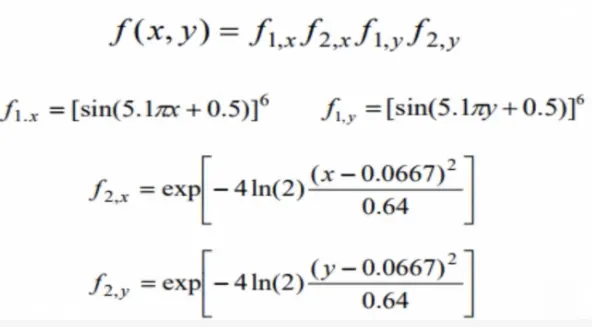
function [f] = stalagmite(input_vector)

x1 = input_vector(1);
y1 = input_vector(2);

f_1x = (sin((5.1*pi*x1)+0.5))^6;
f_2y = (sin((5.1*pi*y1)+0.5))^6;
f_1a = exp((-4*log(2)*(x1-0.0667)^2)/0.64);
f_2b = exp((-4*log(2)*(y1-0.0667)^2)/0.64);

[f] = -(f_1x*f_2y*f_1a*f_2b);
end
MAIN FUNCTION CODE:
clear all
close all
clc

%defining search space

x = linspace(0,0.6,150);
y = linspace(0,0.6,150);

%creating a 2dimensional mesh
[xx, yy] = meshgrid(x,y);

%evaluating the stalagmite function

for i = 1:length(xx)
    for j = 1:length(yy)
        input_vector(1) = xx(i,j);
        input_vector(2) = yy(i,j);
        f(i,j) = stalagmite(input_vector);
        end
end

surfc(xx,yy,-f)

xlabel('x values')
ylabel('y values')

shading interp

[x,fval] = ga(@stalagmite,2)
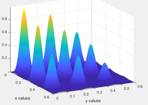
The plot generated is shown below:
STUDY 1 - STATISTICAL STUDY WITHOUT BOUNDATION
- In this evaluating the optimum value of fitness function at each iteration and calculating it using the above mentioned syntax in the intro part
- Then plotting it into the surf command and also providing the optimum values of the function that how its is varying
- Also using the tic and tok command to evaluate the time used for optimizing the function
clear all
close all
clc

%defining our search space

x = linspace(0,0.6,150);
y = linspace(0,0.6,150);
num_cases = 50;

%creating a 2dimensional mesh
[xx, yy] = meshgrid(x,y);

%evaluating the stalagmite function

for i = 1:length(xx)
    for j = 1:length(yy)
        input_vector(1) = xx(i,j);
        input_vector(2) = yy(i,j);
        f(i,j) = stalagmite(input_vector);
        end
end

tic
%study 1-statistical behaviour with unbounded input values

for a = 1:num_cases
    [inputs,fopt_1(a)] = ga(@stalagmite,2)
xopt(a) = inputs(1);
yopt(a) = inputs(2);
end
study1_time = toc

    %plotting data
    figure(1)
    subplot(2,1,1)
    hold on
    surfc(x,y,-f)
    shading interp
    colorbar
    plot3(xopt,yopt,-fopt_1,'marker','o','markerfacecolor','r','markersize',5)
    title('unbounded inputs')
    subplot(2,1,2)
    plot(-fopt_1)
    xlabel('iterations')
    ylabel('function maximum')
RESULTS:
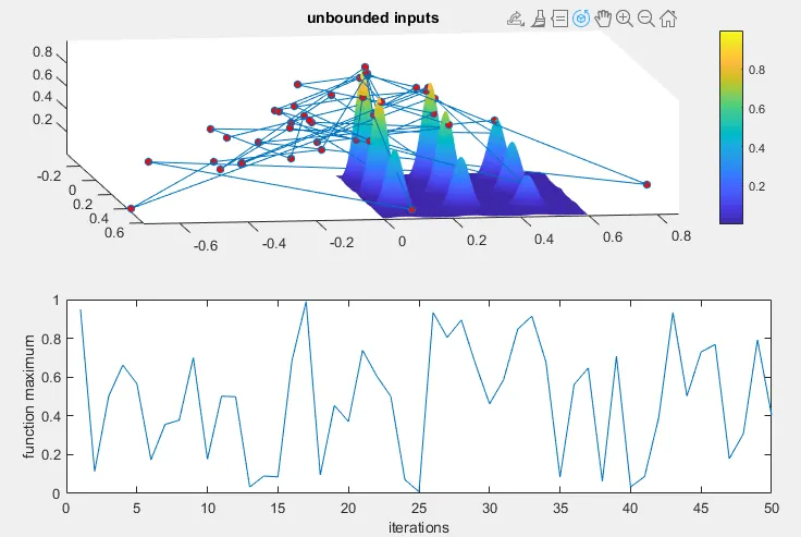
The result is not much accurate and giving a lot of variation in optimizing the function
STUDY 2-STATISTICAL STUDY WITH BOUNDATION:
- The difference over here is in providing the upper and lower limit in ga so that the search space is reduced with the upper and lower boundary
- And the potting it similar as study 1
clear all
close all
clc

%defining our search space

x = linspace(0,0.6,150);
y = linspace(0,0.6,150);
num_cases = 50;

%creating a 2dimensional mesh
[xx, yy] = meshgrid(x,y);

%evaluating the stalagmite function

for i = 1:length(xx)
    for j = 1:length(yy)
        input_vector(1) = xx(i,j);
        input_vector(2) = yy(i,j);
        f(i,j) = stalagmite(input_vector);
        end
end

tic
%study 2-statistical behaviour with unbounded input values

for b = 1:num_cases
    [inputs,fopt_2(b)] = ga(@stalagmite,2,[],[],[],[],[0;0],[0.6;0.6]);
xopt(b) = inputs(1);
yopt(b) = inputs(2);
end
study2_time = toc

    %plotting data
    figure(2)
    subplot(2,1,1)
    hold on
    surfc(x,y,-f)
    shading interp
    colorbar
    plot3(xopt,yopt,-fopt_2,'marker','o','markerfacecolor','r','markersize',5)
    title('bounded inputs')
    subplot(2,1,2)
    plot(-fopt_2)
    xlabel('iterations')
    ylabel('function maximum')
RESULTS:
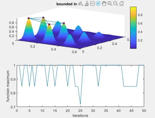
It is clearly seen from the above that after providing the boundary limits the variation in the optimum value of the function has reduced
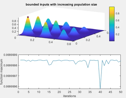
STATISTICAL STUDY WITH INCREASE IN SIZE OF POPULATION:
- In this study using the 'optimoptions'command to increase the size of population.
- the benefit of that will be it will be working on the large set of numbers and which will be led to increase the possibilities of finding the better fittnes of function.
- The draw back is that the time of evaluation will increase
clear all
close all
clc

%defining our search space

x = linspace(0,0.6,150);
y = linspace(0,0.6,150);
num_cases = 50;

%creating a 2dimensional mesh
[xx, yy] = meshgrid(x,y);

%evaluating the stalagmite function

for i = 1:length(xx)
    for j = 1:length(yy)
        input_vector(1) = xx(i,j);
        input_vector(2) = yy(i,j);
        f(i,j) = stalagmite(input_vector);
        end
end

%study 3-statistical behaviour with unbounded input values
%and increasing genetic algorithm iterations

option_1 = optimoptions('ga');
option_1 = optimoptions(option_1,'populationsize',300);

tic
for c = 1:num_cases
    [inputs,fopt_3(c)] = ga(@stalagmite,2,[],[],[],[],[0;0],[1;1],[],[],option_1);
xopt(c) = inputs(1);
yopt(c) = inputs(2);
end
study3_time = toc

    %plotting data
    figure(3)
    subplot(2,1,1)
    hold on
    surfc(x,y,-f)
    shading interp
    colorbar
    plot3(xopt,yopt,-fopt_3,'marker','o','markerfacecolor','r','markersize',5)
    title('bounded inputs with increasing population size')
    subplot(2,1,2)
    plot(-fopt_3)
    xlabel('iterations')
    ylabel('function maximum')
RESULTS:
STUDY TIMES:
- STUDY 1 TIME:5.3466
- STUDY 2 TIME:7.2425
- STUDY 3 TIME:25.2836