Genetic Algorithm

AIM:

To write a code in MATLAB to optimise the stalagmite function and find the global maxima of the function.

THEORY:

The name for the function, Stalagmite is due to the pointy structure of the graph resembling stalagmite rocks.

Genetic algorithm imitates the process of natural selection in the Darwin's theory of evolution. It helps search problems and find the optimum values .

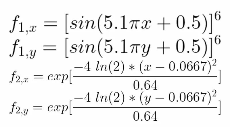
Global minima, F = -(F1*F2*F3*F4)

where F1, F2, F3 & F4 as follows respectively.

PROCEDURE:

Values are assigned to x and y. Then we use linspace commands to create 150 values from 0 to 0.6.

We use meshgrid command to evaluate the functions of two variables and three dimensional plots.

Then stalagmite functions is used for different iterations.

By using GA function, we define stalagmite function for three iterations.

We measure the time for each of the iterations & put more boundary conditions to find the optimum value.

CODE:

clear all
close all
clc

x = linspace(0,0.6,150);
y = linspace(0,0.6,150);
num_cases = 50
f = get_stalagmite(x,y);

tic
%study 1 - statistical behaviour
for i = 1:num_cases
    [inputs, fopt(i)] = ga(@stalagmite, 2);
    xopt(i) = inputs(1);
    yopt(i) = inputs(2);
end

study1_time = toc

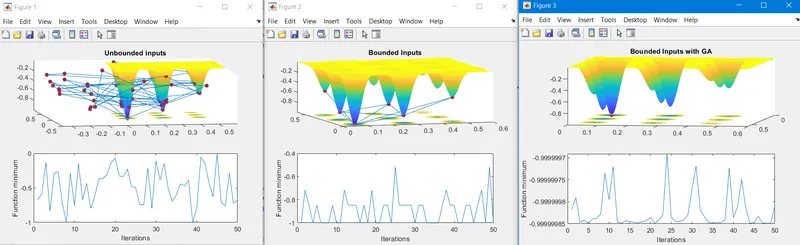
figure(1)
subplot(2,1,1)
hold on
surfc(x,y,f)
shading interp
plot3(xopt, yopt, fopt,'marker','o','markersize',5,'markerfacecolor','r')
title('Unbounded inputs')
subplot(2,1,2)
plot(fopt)
xlabel('Iterations')
ylabel('Function minimum')

tic
%study 2 - Stattistical behaviour - with upper and lower bounds
for i = 1:num_cases
    [inputs, fopt(i)] = ga(@stalagmite,2,[],[],[],[],[0,0],[1,1]);
    xopt(i) = inputs(1);
    yopt(i) = inputs(2);
end
study2_time = toc

figure(2)
subplot(2,1,1)
hold on
surfc(x,y,f)
shading interp
plot3(xopt,yopt,fopt,'marker','o','markersize',5,'markerfacecolor','r')
title('Bounded Inputs')
subplot(2,1,2)
plot(fopt)
xlabel('Iterations')
ylabel('Function minimum')

%study 3 - increasing GA iterations
options = optimoptions('ga');
options = optimoptions(options,'PopulationSize',170);

tic
for i = 1:num_cases
    [inputs, fopt(i)] = ga(@stalagmite,2,[],[],[],[],[0,0],[0.2,0.2],[],[],options);
    xopt(i) = inputs(1);
    yopt(i) = inputs(2);
end
study3_time = toc

figure(3)
subplot(2,1,1)
hold on
surfc(x,y,f)
shading interp
plot3(xopt,yopt,fopt,'marker','o','markersize',5,'markerfacecolor','r')
title('Bounded Inputs with GA')
subplot(2,1,2)
plot(fopt)
xlabel('Iterations')
ylabel('Function minimum')

function [F] = stalagmite(input_vector)

x = input_vector(1);
y = input_vector(2);

F1 = (sin(5.1*pi*x + 0.5)).^6;
F2 = (sin(5.1*pi*y + 0.5)).^6;
F3 = exp(-4*log(2)*(x-0.0667).^2/0.64);
F4 = exp(-4*log(2)*(y-0.0667).^2/0.64);

F = -F1*F2*F3*F4;

end

function f = get_stalagmite(x,y)

num_cases = 50;

%creating a 2D mesh
[xx yy] = meshgrid(x,y);

%Evaluating the stalagmite function
for i = 1:length(xx)
    for j = 1:length(yy)
        input_vector(1) = xx(i,j);
        input_vector(2) = yy(i,j);
        f(i,j) = stalagmite(input_vector);
    end
end
end

CODE EXPLANATION:

Function stalagmite is created using input vectors x and y.

F = stalagmite(input_vector)

Input arrays are stored in x and y

x = input_vector(1)

y = input_vector(2)

Storing x and y values in f using function command

f(i,j) = get_stalagmit(input_vector)

using stalagmite functions equations, we store stalagmite values in funtion, F

F = -F1*F2*F3*F4

Using linspace command, values are assigned to x and y. num_cases used to take 50 cases out of it.

2D array of x & y is created using meshgrid command

Forloop is used to assign variables to input_vector(1) & input_vector(2)

Study time is allocated by a stop watch using tic-toc command.

Genetic algorithm command is used to solve stalagmite function with 2 variables.

Optimum values of x & y are stored in inputs.

Optimum value of f is stored in fopt.

GA finds the global minimas, to find the maximum, we change F to -F.

surfc command is used to create a surface plot of values of f.

3D plot is created by plot3 command.

Options command is used as stopping criteria.

options = optimoptions('ga')

OUTPUT: