FINAL INDEPENDENT PROJECT

PROJECT TITLE: Inverse kinematics of a 2 link Robotic Arm.

AIM : To write a program in MATLAB to simulate the Inverse kinematics of a 2 link Robotic Arm.

THEORY : Inverse kinematics makes use of the kinematic equations to determine the joint parameters that provide a desired configuration (position and rotation) for each of the robot's end effectors.Determining the movement of a robot so that its end-effectors move from an initial configuration to a desired configuration is known as motion planning. Inverse kinematics transforms the motion plan into joint actuator trajectories for the robot.

This is a typical problem in robotics that needs to be solved to control a robotic arm to perform tasks it is designated to do. In a 2-dimensional input space, with a two-joint robotic arm and given the desired coordinate, the problem reduces to finding the two angles involved. The first angle is between the first arm and the ground (or whatever it is attached to). The second angle is between the first arm and the second arm.

Kinematics is the study of motion without considering the cause of the motion, such as forces and torques. Inverse kinematics is a method that helps define the motion of a robot to reach a desired location. For example, to perform a surgical task, a robotic arm used in a medical surgery needs precise motion from an initial location to a desired location.

Robot kinematics involves deriving equations to describe an analytical relationship between the robot’s joint parameters and the tip or end-effector. There are two ways to derive the equations of motion:

1.Forward kinematics - Given the joint angle values, forward kinematics equations calculate the robot’s end-effector location in the coordinate space.

2.Inverse kinematics - Given the robot’s end-effector location, inverse kinematics equations calculate the joint angles required to move the end-effector to that location.

MATLAB CODE :

The program in MATLAB to simulate the Inverse kinematics of a 2 link Robotic Arm.

%giving input lengths of arms
my_L1    = 1;
my_L2    = 0.5; 
syms theta_1 theta_2 L_1 L_2 XE YE
%forward kinematics
the_XE_RHS = L_1*cos(theta_1) + L_2*cos(theta_1 + theta_2)
the_YE_RHS = L_1*sin(theta_1) + L_2*sin(theta_1 + theta_2)
XE_MLF     = matlabFunction(the_XE_RHS, 'Vars', [L_1, L_2, theta_1, theta_2]);
YE_MLF     = matlabFunction(the_YE_RHS, 'Vars', [L_1, L_2, theta_1, theta_2]);
t1_degs_row          = linspace(   0, 90, 1000);
t2_degs_row          = linspace(-180,180, 1000);
[tt1_degs, tt2_degs] = meshgrid(t1_degs_row, t2_degs_row);
tt1_rads  = tt1_degs * pi/180;
tt2_rads  = tt2_degs * pi/180;
my_X_mat   = XE_MLF(my_L1, my_L2, tt1_rads, tt2_rads); 
my_Y_mat   = YE_MLF(my_L1, my_L2, tt1_rads, tt2_rads); 
bh_2dof_plot_XY_given_theta( tt1_degs, tt2_degs, ...
                             my_X_mat, my_Y_mat, ...
                            (my_L1 + my_L2) )
                        
%inverse kinematics
XE_EQ  = XE == the_XE_RHS;
YE_EQ  = YE == the_YE_RHS;
S      = solve([XE_EQ, YE_EQ], [theta_1, theta_2])
simplify( S.theta_1 )
S.theta_2
TH1_MLF{1} = matlabFunction(S.theta_1(1), 'Vars', [L_1, L_2, XE, YE]);
TH1_MLF{2} = matlabFunction(S.theta_1(2), 'Vars', [L_1, L_2, XE, YE]);
TH2_MLF{1} = matlabFunction(S.theta_2(1), 'Vars', [L_1, L_2, XE, YE]);
TH2_MLF{2} = matlabFunction(S.theta_2(2), 'Vars', [L_1, L_2, XE, YE]);
% Here's our mesh of X,Y co-ordinates
[xmat, ymat] = meshgrid([0:0.01:1.5], [0:0.01:1.5]);
% compute inverse kinematics
tmp_th1_mat  = TH1_MLF{1}(my_L1, my_L2, xmat, ymat);
tmp_th2_mat  = TH2_MLF{1}(my_L1, my_L2, xmat, ymat);
% convert to degrees
tmp_th1_mat = (180/pi)*tmp_th1_mat ;
tmp_th2_mat = (180/pi)*tmp_th2_mat ;
% replace imaginary numbers
th1_mat = NaN*ones(size(tmp_th1_mat));
th2_mat = NaN*ones(size(tmp_th2_mat));
tf_mat= imag(tmp_th1_mat)==0;  th1_mat(tf_mat)= real(tmp_th1_mat(tf_mat));
tf_mat= imag(tmp_th2_mat)==0;  th2_mat(tf_mat)= real(tmp_th2_mat(tf_mat));
% plot it
bh_2dof_plot_theta_given_XY( xmat,    
                              ymat,   
                             th1_mat, 
                             th2_mat)

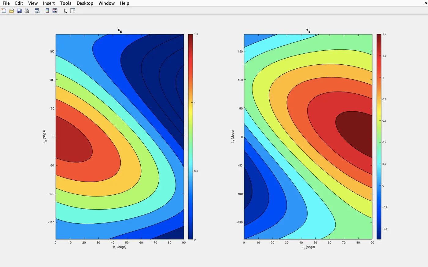
First function to plot XY given the values of theta

function  bh_2dof_plot_XY_given_theta( theta_1_mat_degs, ...
                                  theta_2_mat_degs, ...
                                  X_mat,       ...
                                  Y_mat, ...
                                  a_cmax)
                              
xlab_str = 'theta_1 (degs)';
ylab_str = 'theta_2 (degs)';
figure;
hax(1) = subplot(1,2,1);
   contourf(theta_1_mat_degs, theta_2_mat_degs, X_mat); 
      caxis(hax(1), [0, a_cmax]);
      colormap(gca,'jet'); colorbar
      xlabel(xlab_str, 'Interpreter', 'tex');
      ylabel(ylab_str, 'Interpreter', 'tex');
      title(hax(1), 'X_E', 'Interpreter', 'tex')
hax(2) = subplot(1,2,2);
   contourf(theta_1_mat_degs, theta_2_mat_degs, Y_mat); 
      caxis(hax(1), [0, a_cmax]);
      colormap(gca,'jet'); colorbar
      xlabel(xlab_str, 'Interpreter', 'tex');
      ylabel(ylab_str, 'Interpreter', 'tex');
      title(hax(2), 'Y_E', 'Interpreter', 'tex')
end

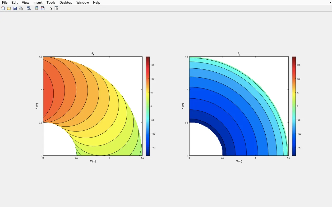
Second function to plot theta given XY

function  bh_2dof_plot_theta_given_XY( X_mat,       ...
                                       Y_mat, ...
                                       theta_1_mat_degs, ...
                                       theta_2_mat_degs)
                              
xlab_str = 'X (m)';
ylab_str = 'Y (m)';
hfig = figure;
hax(1) = subplot(1,2,1);
   contourf(X_mat, Y_mat, theta_1_mat_degs); 
      caxis(hax(1), [-180, 180]);
      colormap(gca,'jet'); colorbar
      xlabel(xlab_str, 'Interpreter', 'tex');
      ylabel(ylab_str, 'Interpreter', 'tex');
      title(hax(1), 'theta_1', 'Interpreter', 'tex')
      axis('equal')
hax(2) = subplot(1,2,2);
   contourf(X_mat, Y_mat, theta_2_mat_degs); 
      caxis(hax(2), [-180, 180]);
      colormap(gca,'jet'); colorbar
      xlabel(xlab_str, 'Interpreter', 'tex');
      ylabel(ylab_str, 'Interpreter', 'tex');
      title(hax(2), 'theta_2', 'Interpreter', 'tex')
      axis('equal')
      
end

TERMINOLOGY USED : 

1.linspace : linspace is similar to the colon operator, “:”, but gives direct control over the number of points and always includes the endpoints. “lin” in the name “linspace” refers to generating linearly spaced values as opposed to the sibling function logspace, which generates logarithmically spaced values.

EXPLANATION :

1. First define the geometry parameters 

my_L1 = 1;

APPLICATION :

1.Inverse kinematics is also used to recover the movements of an object in the world from some other data, such as a film of those movements, or a film of the world as seen by a camera which is itself making those movements.

2.Game programming and 3D animation - Inverse kinematics is important to game programming and 3D animation, where it is used to connect game characters physically to the world, such as feet landing firmly on top of terrain.

3.Interactive manipulation : Interactive application involving human characters that can autonomously manipulate objects. The software is able to generate collision-free motions for typical single-arm manipulation tasks at interactive rates. 

4.Collision avoidance : Collision detection is the computational problem of detecting the intersection of two or more objects. While collision detection is most often associated with its use in video games and other physical simulations, it also has applications in robotics. In addition to determining whether two objects have collided, collision detection systems may also calculate time of impact (TOI), and report a contact manifold (the set of intersecting points).

5.Medical surgery - To perform a surgical task, a robotic arm used in a medical surgery needs precise motion from an initial location to a desired location.

OBSERVATION : 

For the FORWARD kinematics we get 2 plots , one for XE and other for YE.(i.e to plot XY given the values of theta. )

For the INVERSE kinematics we get 2 plots , one for XE and other for YE.(i.e to plot theta given XY.)

RESULT : The simulation of the Inverse kinematics of a 2 link Robotic Arm is done and plotted using MATLAB and the practical applications and importance of it is detailed in the report.