Project 1 - Parsing NASA thermodynamic data
AIM:
- To write a code in MATLAB to parse nasa thermodynamic data file and then calculate thermodynamic properties of various gas species.
- Write a function that extracts the 14 coefficients and calculates the enthalpy,entropy and specific heats for all the species in the data file.
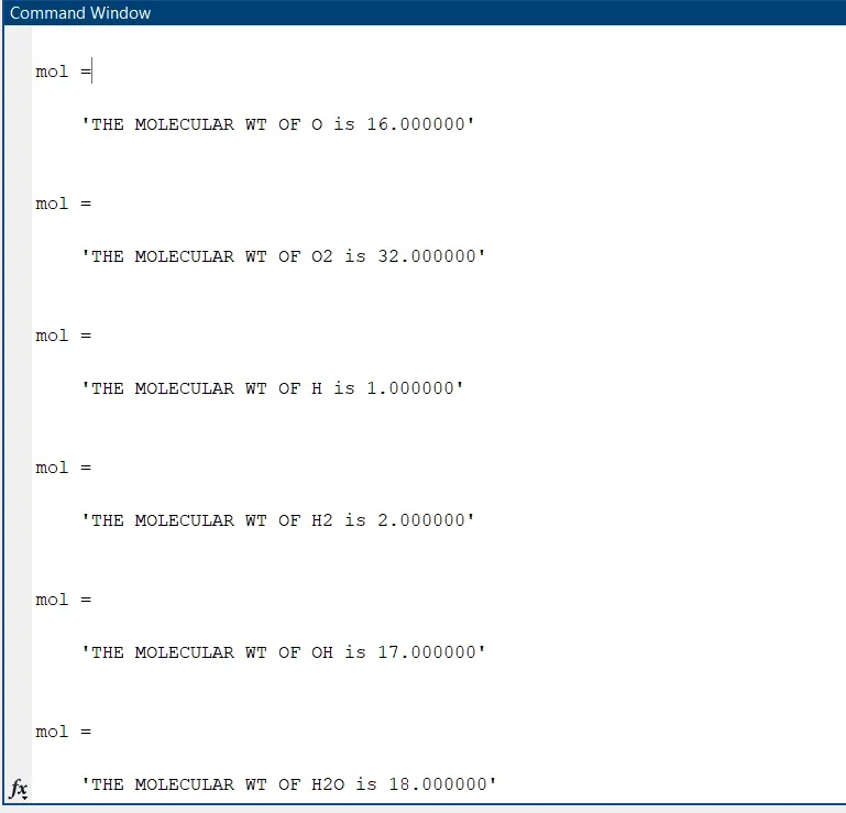
- Calculating molecular weight of each species.
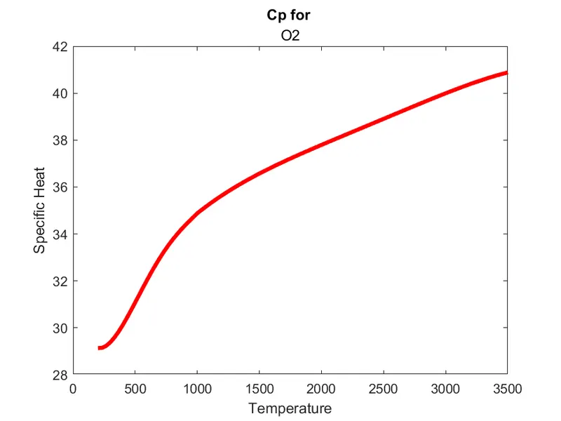
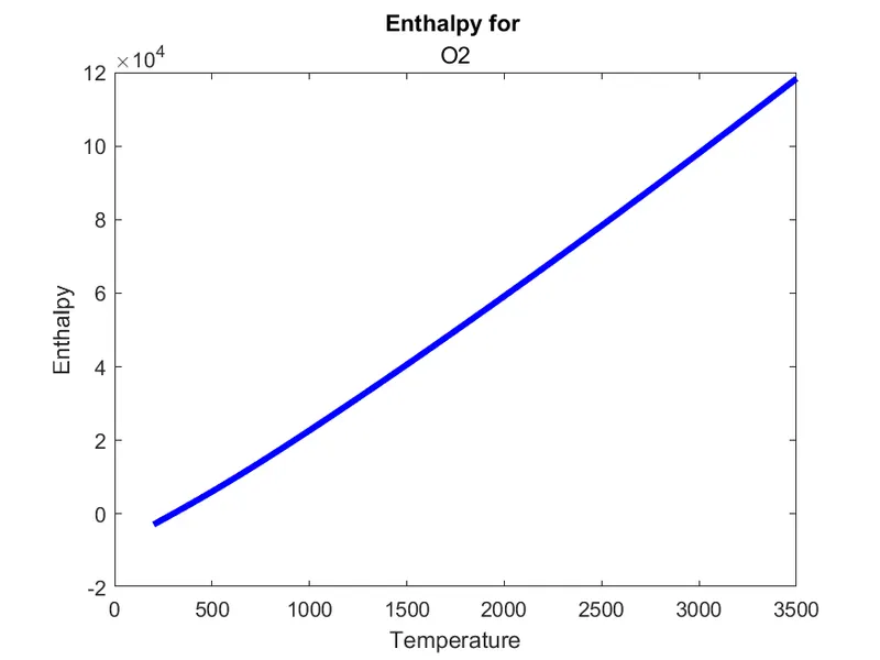
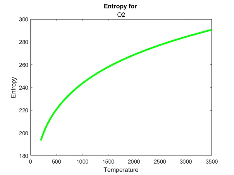
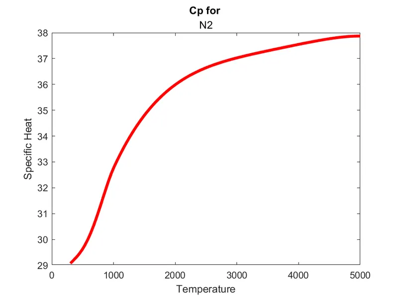
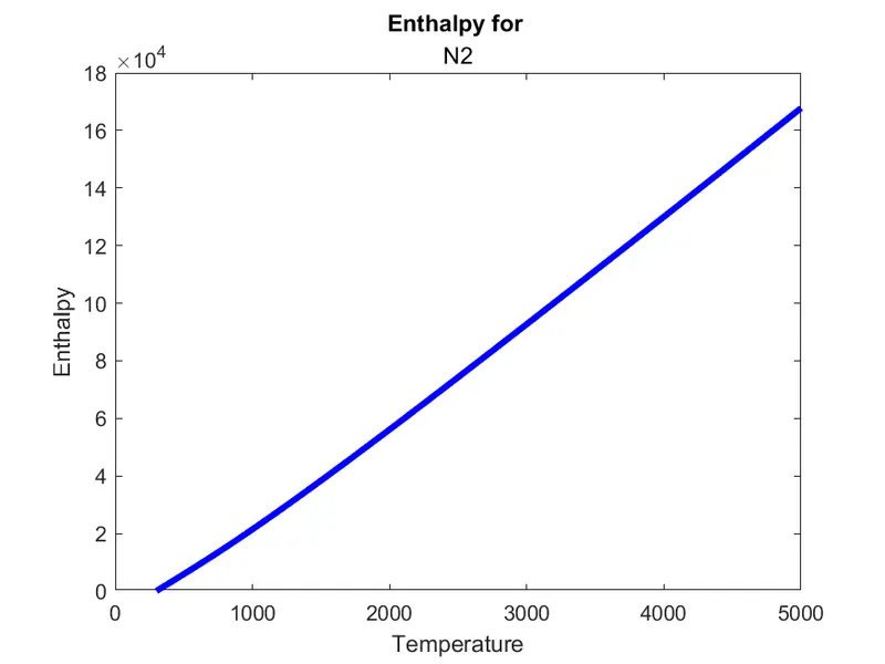
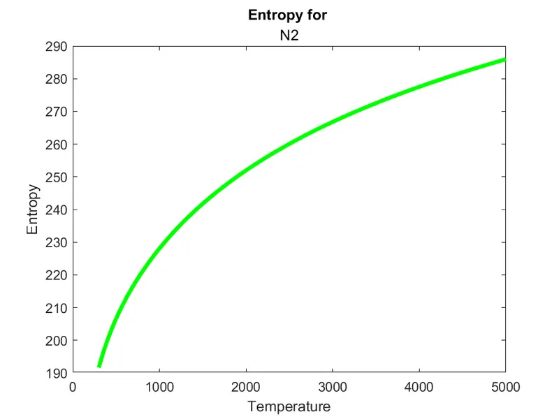
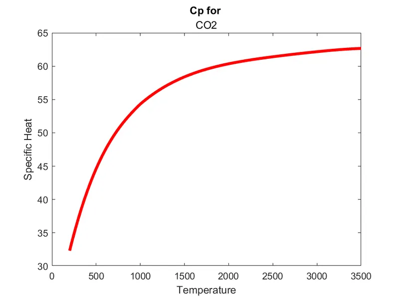
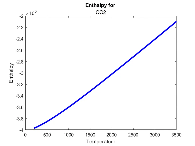
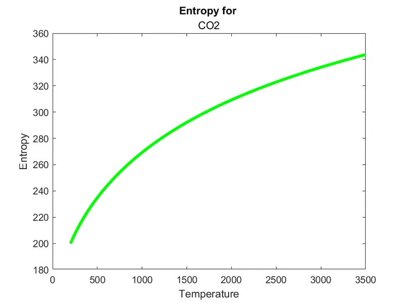
- Plotting the specific heat,enthalpy and entropy for the local temperature range.
- Saving the plots as images with appropriate names and dumping them in seperate folders for each species.
THEORY:
File Parsing
File parsing is reading and analyzing string or text in a data stream of some sort and building an in memory model of the semantic content of that data.
For specific heat

For enthalpy

For entropy

where
T=local temprature
b1-b7=high temperature coefficient
b8-b14=low temprature coefficient
R=Gas constant=8.314
CODE:
% Reading the NASA thermo.dat file
clear all
close all
clc

f1=fopen('THERMO.dat','r');

%reading header information
fgetl(f1);
%global temperature
t_line= fgetl(f1) ;

%splitting with space
a=strsplit(t_line,' ');

global_low_temp=str2double(a{1});
global_mid_temp=str2double(a{2});
global_high_temp=str2double(a{3});

%ignoring the 3 lines
fgetl(f1);
fgetl(f1);
fgetl(f1);

%reading species block
%line 1
for i=1:53
    t_line2=fgetl(f1);
    s=strsplit(t_line2,' ');
    species_name=s{1};
    A=strfind(t_line2,'G');
    temp_values=t_line2(A+4:length(t_line2));
    B=strsplit(temp_values,' ');

    local_low_temp=str2double(B{1});
    local_mid_temp=str2double(B{3});
    local_high_temp=str2double(B{2});

    %line after species line
    t_line= fgetl(f1);
    b=findstr(t_line,'E');
    %1st coefficient
    b1=t_line(1:b(1)+3);
    b1=str2num(b1);
    %2nd coefficient
    b2=t_line(b(1)+4:b(2)+3);
    b2=str2num(b2);
    %3rd coefficient
    b3=t_line(b(2)+4:b(3)+3);
    b3=str2num(b3);
    %4th coefficient
    b4=t_line(b(3)+4:b(4)+3);
    b4=str2num(b4);
    %5th coefficient
    b5=t_line(b(4)+4:b(5)+3);
    b5=str2num(b5);

    %line 2
    line2=fgetl(f1);
    b=findstr(line2,'E');
    %6th coefficient
    b6=line2(1:b(1)+3);
    b6=str2num(b6);
    %7th coefficient
    b7=line2(b(1)+4:b(2)+3);
    b7=str2num(b7);
    %8th coefficient
    b8=line2(b(2)+4:b(3)+3);
    b8=str2num(b8);
    %9th coefficient
    b9=line2(b(3)+4:b(4)+3);
    b9=str2num(b9);
    %10th coefficient
    b10=line2(b(4)+4:b(5)+3);
    b10=str2num(b10);

    %line 3
    line3=fgetl(f1);
    b=findstr(line3,'E');
    %11th coefficient
    b11=line3(1:b(1)+3);
    b11=str2num(b11);
    %12th coefficient
    b12=line3(b(1)+4:b(2)+3);
    b12=str2num(b12);
    %13th coefficient
    b13=line3(b(2)+4:b(3)+3);
    b13=str2num(b13);
    %14th coefficient
    b14=line3(b(3)+4:b(4)+3);
    b14=str2num(b14);


%     mkdir(species_name)
%     cd(species_name)
%
%     %universal gas constant
    R=8.314;

    t=linspace(local_low_temp,local_high_temp,100);

    for i = 1:length(t)
    if t(i)>=1000
        %Specific Heat
        Cp(i) = R*(b1 + b2*t(i) + b3*t(i).^2 + b4*t(i).^3 + b5*t(i).^4);
        %Enthalpy
        H(i) = R*t(i)*(b1 + (b2*t(i))./2 + (b3*t(i).^2)./3 + (b4*t(i).^3)./4 + (b5*t(i).^4)./5 + b6/t(i));
        %Entropy
        S(i) = R*(b1*log(t(i)) + b2*t(i) + (b3*t(i).^2)./2 + (b4*t(i)^3)./3 + (b5*t(i).^4)/4 + b7);

    else
         Cp(i) = R*(b8 + b9*t(i) + b10*t(i).^2 + b11*t(i).^3 + b12*t(i).^4);
         H(i) = R*t(i)*(b8 + (b9*t(i))./2 + (b10*t(i).^2)/3 + (b11*t(i).^3)/4 + (b12*t(i).^4)./5 + b13/t(i));
         S(i) = R*(b8*log(t(i)) + b9*t(i) + (b10*t(i).^2)/2 + (b11*t(i).^3)/3 + (b12*t(i).^4)/4 + b14);
    end
    end

    figure(1)
    plot(t,Cp,'linewidth',3,'color','r')
    xlabel('Temperature')
    ylabel('Specific Heat')
    title('Cp for ',species_name)
    saveas(1,'Cp_vs_T.png')

    figure(2)
    plot(t,H,'linewidth',3,'color','b')
    xlabel('Temperature')
    ylabel('Enthalpy')
    title('Enthalpy for ',species_name)
    saveas(2,'H_vs_T.png')

    figure(3)
    plot(t,S,'linewidth',3,'color','g')
    xlabel('Temperature')
    ylabel('Entropy')
    title('Entropy for ',species_name)
    saveas(3,'S_vs_T.png')

    cd ..


  %mol wt calc
  %primary elements
    elements=['H','C','O','N','A'];
%element names for comparison
    atomic_wt=[1 12 16 14 40];
%weight assigned for each element
    mol_wt=0;
    for k=1:length(species_name)
        for l=1:length(elements)
            %string comparison
            if strcmp(species_name(k),elements(l))
%comparison of the characters, and proceed if yes
                mol_wt=mol_wt+atomic_wt(l);
                position=l;
                %storing the position for reference outside loop

            end

        end

   %str2num
       n=str2double(species_name(k));

         if (n>1)
        mol_wt= mol_wt+atomic_wt(position)*(n-1);
        % adding the extra atoms' weights

         end
    end

      mol=sprintf('THE MOLECULAR WT OF %s is %f',species_name,mol_wt)


end
EXPLAINATION:
- The program begins with clear all, close all and clc which clears the workspace, closes all the plots and clears the command window respectively.
- In the next step, NASA thermodat file is opened using the command fopen. the letter r after the file indicates read mode.
- Using the fgetl command, we extract each line of the file into the command window. The first line being the header info followed by global temperature values.The next three lines are comments which are not required from program point of view.
- The global temperature values obtained in the previous step is in the form of strings. In order to convert them into numbers, str2num command is used.
- From the 6th line onwards, we have the 53 species name and their 14 coefficients. Using the for loop, the name of the species and its coefficients are extracted.
- The first fgetl command in the loop gets us the species name.
- The next three fget helps us extract the coefficient values.
- The strfind command helps us to locate the letter E(exponential) which is used as reference for gettiing the coefficient values. These values extracted as strings are then converted into numbers using str2num command.
- The mkdir command creates a folder for saving the plots that will be generated.
- A range of temperature is assumed for calculating enthalpy,entropy and specific heat values.
- In the next step, the for loop determines these parameters for each temperature values.
- With the help of plot command, the calculated parameters are plotted against the corresponding value of temperature.
- The file directory is then changed to the one that was created in the 9th step to save these plots.
- Saveas command helps us in saving these plots with the names we want.
- The directory is then switched back for molecular mass calculation.
- Next line is a function call to calculate the molecular mass.
- This function takes species_name as input and gives out its Molecular mass as output.
- Each species name is stored in a string called species.
- From the file given, it can be seen that the constituents that make up each species are Hydrogen(H), Carbon(C), Nitrogen(N), Oxygen(O) and Argon(Ar). So the starting letter of each element is stored as constituents .
- The atomic weights of each constituent is stored in an array called atomic_weight.
- The molecular weight is set to zero in the beginning,
- Using the nested for loop, molecular weight is calculated as follows:
- The first for loop runs for entire length of species name that has been determined by the for loop in the main program.
- The second for loop runs for entire length of constituent array.
- Using the strcmp command which compares2strings and returns 1 if they match, the molecular weight will be incremented by the corresponding value in the array'atomic_weight'.
- Another if statement checks if a molecule in a specie has more than one molecule and increases its molecular weight correspondingly.
OUTPUT:
Screenshot of Saved Files

Plots for O2
Plots for N2
Plots for Co2
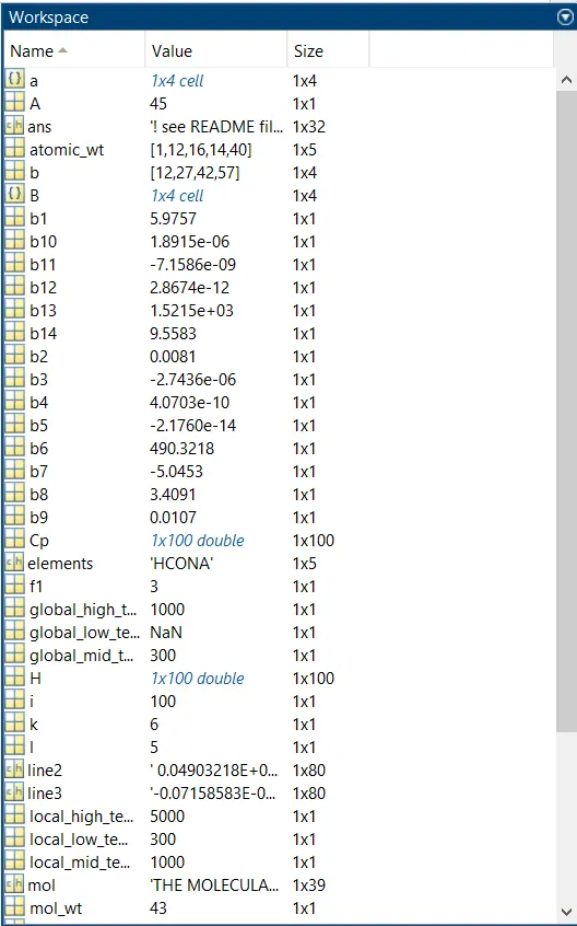
Workspace:
Molecular Weight: