Week 3 - Solving second order ODEs

AIM:

To write a program that solves ODE representing the equation of motion of a simple pendulum with damping.

To create animation motion of the pendulum by the position of the pendulum as a function of time.

THEORY:

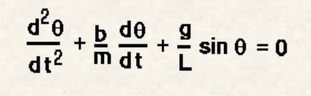
This 2nd order ODE represents the equation of motion of a simple pendulum with damping.

g = gravity in m/s2,

L = length of the pendulum in m,

m = mass of the ball in kg,

b=damping coefficient.

By solving the equation with ode45 function, we will simulate the motion of the pendulum.

PROCEDURE:

We give initial inputs to the variables in the ODE.

L=1 metre,

m=1 kg,

b=0.05.

g=9.81 m/s2.

We take time from 0-20 sec

and angular displacement=0, angular velocity=3 rad/sec at time t=0.

When you do this you will get the position of the pendulum as a function of time.This information is used to animate the motion of the pendulum.

• Initially we solve the 2nd order ODE equation with ode45 & function syntax..
• Then for each value in time, we create an image that represents the position of the pendulum by plot command
• We use the marker command to create a sphere
• One end of the pendulum is fixed & we plot a fixed axis.
• The other end moves according to the solution of the ODE we had solved.
• Then we use the movie command create an animation.

CODE:

close all
clear all
clc

% inputs
b=0.05;
g=9.81;
l=1;
m=1;

%initial condition
theta_0 = [0;3]

%time points
t_span = linspace(0,20,150)

%solve ODE
[t, results] = ode45(@(t,theta) ode_func(t, theta, b,g,l,m),t_span,theta_0);

figure(1)
plot(t,results(:,1))
hold on
plot(t,results(:,2))
ylabel('Plot')
xlabel('TIme')
legend('Displacement','Velocity')

theta = results(:,1);

ct=1;
for i = 1:length(theta);
    THETA = theta(i);
    
    x0 = 0;
    y0 = 0;
    
    x1 = l*sin(THETA);
    y1 = -l*cos(THETA);
    
    figure(2)
    plot([-1.5,1.5],[0,0])
    hold on
    plot([x0,x1],[y0,y1],'linewidth',3)
    hold on
    plot(x1,y1,'o','markersize',20,'markerfacecolor','r')
    axis([-1 1 -1.5 1.5])
    hold off
     
    M(ct) = getframe(gcf)
    ct = ct+1
end

movie(M)
videofile = VideoWriter('ODE_pendulam','uncompressed AVI')
open(videofile)
writeVideo(videofile,M)
close(videofile)

function [dtheta_dt] = ode_func(t,theta,b,g,l,m)

theta1 = theta(1)
theta2 = theta(2)
dtheta1_dt = theta2;
dtheta2_dt = -(b/m)*theta2 - (g/l)*sin(theta1);
dtheta_dt = [dtheta1_dt; dtheta2_dt];
end

CODE EXPLANATION:

Initially we give the inputs for variables in the ODE equation.

And now we assume initial condtions with displacement = 0 rad, time = 0 sec and velocity = 3 rad/sec.

Then the time period is taken from 0 to 20 sec and we choose 150 points in this time period to find the motion of pendulum.

Using function, we call values for theta, theta1 and theta2 into the ode45 equation and find the time, displacement & velocity at each of the 150 points in the 0 to 20 sec time frame.

This inturn is plotted in a graph using Plot, legend, axis & marker commands.

To create animation of the motion of pendulum, we again use forloop command to give values for THETA and use Movie command to stimulate and save the animation video.

OUTPUTS:

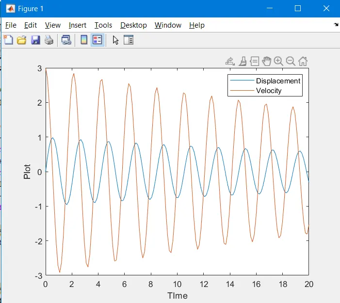
Plot of Displacement & Velocity according to Time.

Animation of pendulum:

https://drive.google.com/file/d/1mXb7a2FfTaCXgW3OMbrxxp7vH8ouOYAr/view?usp=sharing