Week 4 - Genetic Algorithm
1. AIM
- optimisation of stalagmite function using genetic algorithm in matlab
2. OBJECTIVE
- explain the concept of genetic algorithm
- optimize the stalagmite function and find the gloabal maxima
3. THEORY
-stalagmite is ais a type of rock formation that rises from the floor of a cave due to the accumulation of material deposited on the floor from ceilings drippings. Stalagmites are typically composed of calcium carbonate, but may consist of lava, mud, peat, pitch, sand, sinter and amberat.
- stalagmite function is generally refers to the function with which we are generating values over a stalagmite kind of surface for finding out the local and global maxima and minima of that particular given function
- GENETIC ALGORITHM
A genetic algorithm (GA) is a method for solving both constrained and unconstrained optimization problems based on a natural selection process that mimics biological evolution. The algorithm repeatedly modifies a population of individual solutions. At each step, the genetic algorithm randomly selects individuals from the current population and uses them as parents to produce the children for the next generation. Over successive generations, the population "evolves" toward an optimal solution.
GENETIC ALGORITHM FLOW CHART
4. GENETIC ALGORITHM WORKING PROCESS
1. . POPULATION INITILIZATION
. Population is the number of sample data points taken to perform the genetic algorithm operation
2. SELECTION
In this step, the parents are selected from the sample data points, the main objective of the selection process is to select the highly fit individuals.
3. CROSS OVER
It is the process of taking two parents' solutions and producing the child from them
4. MUTATION
Mutation is carried out to maintain the genetic diversity from one generation of a population of chromosomes to the next.
If mutation is not performed, the chromosomes will become too similar to each other, convergence takes place soon and results in local minima.
5. FITNESS FUNCTION
Fitness function takes the solution as input and produces the suitability of the solution as the output. This evaluates how close the solution is to the optimal solution of the desired problem.
6. STOPPING CRITERIA
The algorithm stops when one of the stopping criteria is met.
5. SYNTAX OF GA IN MATLAB
6. CODE EXPLANATION
PROGRAM TO OPTIMISE THE STALAGMITE FUNCTION AND FIND GLOBAL MAXIMA OF THE FUNCTION
CODE EXPLANATION
-in this two arrays x and y are generated in which 150 elements are generated bw 0 and 0.6
- a 2 dimensional array xx and yy is generated using meshgrid command using x and y vectors
- code to evaluate the meshgrid function is coded
- The function stalagmite takes the values from input_vector as inputs and equates and returns the value and stores them in an array 'f'
- commands are given to display the surface plot and to enhance the graphic details on the graph and other details to display
- gentic algorithum code is run
clear all
close all
clc
%defining our search space
x = linspace(0,0.6,150) // commad to create 1dimensional array "x" with values in bw 0 and 0.6 in 150parts
y = linspace(0,0.6,150) // commad to create 1dimensional array "y" with values in bw 0 and 0.6 in 150parts
%creating 2Dimensional array
[xx yy]= meshgrid(x,y);// transforms the domain specified by vectors x and y into arrays xx and yy
% evaluating the meshgrid function
for i=1:length(xx) // for loop and counter variable that will have initial value of 1 to the length or no of elemnets in the array xx that keeps on changing everytime as itloops or executes
for j=1:length(yy)// for loop and counter variable that will have initial value of 1 to the length or no of elemnets in the array yy that keeps on changing everytime as itloops or executes
input_vector(1)= xx(i,j);// creating an array, input_vector(1) which gets value from array xx(i,j) depending upon the location of the pointer variables (i,j) that points out the location on the array depending upon which the variable input_vector(1) will carry the value
input_vector(2)= yy(i,j);// creating an array input_vector(2) gets value from array xx(i,j) depending upon the location of the pointer variables (i,j) that points out the location on the array depending upon which the variable input_vector(2) will carry the value
f(i,j)=stalagmite(input_vector);// an array 'f' which stores the values which are calculated by the function 'stalagmite', which takes in the input_vector as its input variables
end
end
surfc(xx,yy,-f)// command to generate a three-dimensional surface plot with a contour plot underneath. The function plots the values in matrix f as heights above a grid in the x-y plane defined by xx and yy. The color of the surface varies according to the heights specified by f.
-ve sign is used to invert the graph and also If the algorithm is for solving a minimization problem, it can be easily changed to a maximization problem by multiplying the objective function by − 1 and vice versa.
xlabel('x value')// command to label on x-axis
ylabel('y value')// command to label on Y-axis
shading interp // command to remove the grid lines from the graph
[inputs, fval] = ga(@stalagmite,2)// running genetic algorithum code, @stalagmite is the function handle, defines which function is to be minimised and '2' represents the no of variables as inputs in the function, fval stores the value that the function generates
// -code to evaluate the statistical behaviour of the ga code
-in this the search space of the ga code is not specified( boundaries not specified)
-the no of iterations to be performed is defined
- for each iteration process and the value generated by the function, its fitness is evaluated by the
%study1 statistical behaviour
- in this method the search space is not defined or unbounded, only the evaluation of the function is carried out and plotted
- the time taken by this method is evaluated
tic// tic and toc command will calculated the time taken by this particular process( study1),
tic command will initate the timer
num_cases=50 // determines how much time the ga code should repeat or the iteration
for i = 1:num_cases// looping variable for the iteration process
[inputs,fopt(i)]= ga(@stalagmite,2); fopt stores the value of the function that the function generates
xopt(i)= inputs(1);// stores the x-values that the function generates
yopt(i)= inputs(2);// stores the y-values that the function generates
end
study1_time = toc// toc command will stop the timer, command to display the time taken for the processing
// command to plot the graph and labelling
figure(2)
subplot(2,1,1)// to create multiple plots in the figure window
hold on
surfc(x, y,-f)
xlabel('x value')
ylabel('y value')
shading interp
plot3(xopt,yopt,-fopt,'marker','o','markersize',5,'markerfacecolor','r')
title('unbounded inputs')
subplot(2,1,2)
plot(-fopt)
xlabel('iterations')
ylabel('function minimum')
tic
% study2= statistical behaviour - with upper and lower bounds
- in this method the serach space is optimised as we define bounds for the search space, upper limit and lower limit is defined
-time taken by the process is noted
for i = 1:num_cases
[inputs,fopt(i)]= ga(@stalagmite,2,[],[],[],[],[0;0],[1;1]); //
xopt(i)= inputs(1);
yopt(i)= inputs(2);
end
study2_time = toc
// command to plot the graph and labelling
figure(3)
subplot(2,1,1)
hold on
surfc(x, y,-f)
xlabel('x value')
ylabel('y value')
shading interp
plot3(xopt,yopt,-fopt,'marker','o','markersize',5,'markerfacecolor','r')
title('bounded inputs')
subplot(2,1,2)
plot(-fopt)
xlabel('iterations')
ylabel('function minimum')
%study3 - increasing GA iterations
- the search space is defined, uppper and lower limits
- the initial population size is changed
options = optimoptions('ga');
options = optimoptions(options,'populationSize',200);// command increases the population size to 200
for i = 1:num_cases
[inputs,fopt(i)]= ga(@stalagmite,2,[],[],[],[],[0;0],[1;1],[],[],options);
xopt(i)= inputs(1);
yopt(i)= inputs(2);
end
study3_time = toc
// command to plot the graph and labelling
figure(4)
subplot(2,1,1)
hold on
surfc(x, y,-f)
xlabel('x value')
ylabel('y value')
shading interp
plot3(xopt,yopt,-fopt,'marker','o','markersize',5,'markerfacecolor','r')
title('unbounded inputs')
subplot(2,1,2)
plot(-fopt)
xlabel('iterations')
ylabel('function minimum')
STALAGMITE FUNCTION
-inputs are x and y, which are provided by the main function
-this function generates the value of f as the value fo the inputs vary and will evaluate the fitness of the value generated during each iteration
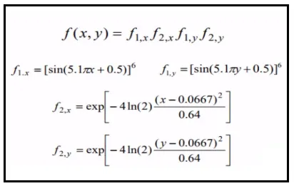
function[f]= stalagmite(input_vector)
x = input_vector(1);
y = input_vector(2);
f1 = [sin(5.1*pi*x+0.5)]^6;
f2 = [sin(5.1*pi*y+0.5)]^6;
f3 = exp(-4*log(2)*(x-0.667)^2/0.64);
f4 = exp(-4*log(2)*(y-0.667)^2/0.64);
f= -(f1*f2*f3*f4);
end
7. CODE
function[f]= stalagmite(input_vector)

x = input_vector(1);
y = input_vector(2);

f1 = (sin(5.1*pi*x+0.5))^6;
f2 = (sin(5.1*pi*y+0.5))^6;
f3 = exp(-4*log(2)*(x-0.667)^2/0.64);
f4 = exp(-4*log(2)*(y-0.667)^2/0.64);

f = -(f1*f2*f3*f4);

end
clear all
close all
clc

%defining our search space
x = linspace(0,0.6,150);
y = linspace(0,0.6,150);
num_cases = 50;


%creating 2Dimensional array
[xx yy]= meshgrid(x,y);

%evaluating the meshgrid function
for i = 1:length(xx)
    for j = 1:length(yy)
        input_vector(1)= xx(i,j);
        input_vector(2)= yy(i,j);
        f(i,j)= stalagmite(input_vector);
    end
end
figure(1)
surfc(xx,yy,-f)
xlabel('x value')
ylabel('y value')

shading interp

[inputs, fval] = ga(@stalagmite,2)


%study1 statistical behaviour

tic
for i = 1:num_cases
    [inputs,fopt(i)]= ga(@stalagmite,2);
    xopt(i)= inputs(1);
    yopt(i)= inputs(2);
end
study1_time = toc

figure(2)
subplot(2,1,1)
hold on
surfc(x, y,-f)
xlabel('x value')
ylabel('y value')
shading interp
plot3(xopt,yopt,-fopt,'marker','o','markersize',5,'markerfacecolor','r')
title('unbounded inputs')
subplot(2,1,2)
plot(-fopt)
xlabel('iterations')
ylabel('function minimum')

tic
% study2= statistical behaviour - with upper and lower bounds

for i = 1:num_cases
    [inputs,fopt(i)]= ga(@stalagmite,2,[],[],[],[],[0;0],[1;1]);
    xopt(i)= inputs(1);
    yopt(i)= inputs(2);
end
study2_time = toc

figure(3)
subplot(2,1,1)
hold on
surfc(x, y,-f)
xlabel('x value')
ylabel('y value')
shading interp
plot3(xopt,yopt,-fopt,'marker','o','markersize',5,'markerfacecolor','r')
title('bounded inputs')
subplot(2,1,2)
plot(-fopt)
xlabel('iterations')
ylabel('function minimum')

%study3 - increasing GA iterations

options = optimoptions('ga');
options = optimoptions(options,'populationSize',200);

for i = 1:num_cases
    [inputs,fopt(i)]= ga(@stalagmite,2,[],[],[],[],[0;0],[1;1],[],[],options);
    xopt(i)= inputs(1);
    yopt(i)= inputs(2);
end
study3_time = toc

figure(4)
subplot(2,1,1)
hold on
surfc(x, y,-f)
xlabel('x value')
ylabel('y value')
shading interp
plot3(xopt,yopt,-fopt,'marker','o','markersize',5,'markerfacecolor','r')
title('unbounded inputs')
subplot(2,1,2)
plot(-fopt)
xlabel('iterations')
ylabel('function minimum')
8. REFERENCES
- https://in.mathworks.com/help/gads/ga.htm
- https://in.mathworks.com/discovery/genetic-algorithm.html
- https://skill-lync.com/knowledgebase/genetic-algorithm-explained