Challenge

Genetic Algorithm - Finding the global maximum of a Stalagmite Function.

MMuthavarapu Chaitanya Krishna8 Jan 2021

AIM: To optimize the stalagmite function and find the global maxima of the function.

OBJECTIVES:

To explain the concept of Genetic Algorithm and the syntax of ‘ga’ in MATLAB.
To find the global maxima of the stalagmite function using genetic algorithm.
To plot graphs for various cases.

THEORY:

Genetic Algorithms (GAs) are search based algorithms based on the concepts of natural selection and genetics. GAs are a subset of a much larger branch of computation known as Evolutionary Computation.

In GAs, we have a pool or a population of possible solutions to the given problem. These solutions then undergo recombination and mutation (like in natural genetics), producing new children, and the process is repeated over various generations. Each individual (or candidate solution) is assigned a fitness value (based on its objective function value) and the fitter individuals are given a higher chance to mate and yield more “fitter” individuals. This is in line with the Darwinian Theory of “Survival of the Fittest”.

In this way we keep “evolving” better individuals or solutions over generations, till we reach a stopping criterion.

Genetic Algorithms are sufficiently randomized in nature, but they perform much better than random local search (in which we just try various random solutions, keeping track of the best so far), as they exploit historical information as well.

Advantages of GAs:

GAs have various advantages which have made them immensely popular. These include −

Does not require any derivative information (which may not be available for many real-world problems).
Is faster and more efficient as compared to the traditional methods.
Has very good parallel capabilities.
Optimizes both continuous and discrete functions and also multi-objective problems.
Provides a list of “good” solutions and not just a single solution.
Always gets an answer to the problem, which gets better over the time.
Useful when the search space is very large and there are a large number of parameters involved.

Limitations of GAs:

Like any technique, GAs also suffer from a few limitations. These include −

GAs are not suited for all problems, especially problems which are simple and for which derivative information is available.
Fitness value is calculated repeatedly which might be computationally expensive for some problems.
Being stochastic, there are no guarantees on the optimality or the quality of the solution.
If not implemented properly, the GA may not converge to the optimal solution.

This notion can be applied for a search problem. We consider a set of solutions for a problem and select the set of best ones out of them. Following phases are considered in a genetic algorithm:

Population:

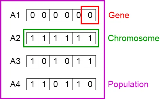
Population is a subset of solutions in the current generation. It can also be defined as a set of chromosomes.

Fitness Function:

The fitness function simply defined is a function which takes a candidate solution to the problem as input and produces as output how “fit” our how “good” the solution is with respect to the problem in consideration.

Calculation of fitness value is done repeatedly in a GA and therefore it should be sufficiently fast. A slow computation of the fitness value can adversely affect a GA and make it exceptionally slow.

In most cases the fitness function and the objective function are the same as the objective is to either maximize or minimize the given objective function. However, for more complex problems with multiple objectives and constraints, an Algorithm Designer might choose to have a different fitness function.

A fitness function should possess the following characteristics −

The fitness function should be sufficiently fast to compute.
It must quantitatively measure how fit a given solution is or how fit individuals can be produced from the given solution.

Parent Selection:

Parent Selection is the process of selecting parents which mate and recombine to create off-springs for the next generation. Parent selection is very crucial to the convergence rate of the GA as good parents drive individuals to a better and fitter solutions.

However, care should be taken to prevent one extremely fit solution from taking over the entire population in a few generations, as this leads to the solutions being close to one another in the solution space thereby leading to a loss of diversity. Maintaining good diversity in the population is extremely crucial for the success of a GA. This taking up of the entire population by one extremely fit solution is known as premature convergence and is an undesirable condition in a GA.

Crossover:

The crossover operator is analogous to reproduction and biological crossover. In this more than one parent is selected and one or more off-springs are produced using the genetic material of the parents. Crossover is usually applied in a GA with a high probability.

Mutation:

In simple terms, mutation may be defined as a small random tweak in the chromosome, to get a new solution. It is used to maintain and introduce diversity in the genetic population and is usually applied with a low probability – p_m. If the probability is very high, the GA gets reduced to a random search.

Mutation is the part of the GA which is related to the “exploration” of the search space. It has been observed that mutation is essential to the convergence of the GA while crossover is not.

Termination:

The algorithm terminates if the population has converged (does not produce offspring which are significantly different from the previous generation). Then it is said that the genetic algorithm has provided a set of solutions to our problem.

Usually, we keep one of the following termination conditions (stopping criteria)−

When there has been no improvement in the population for X iterations.
When we reach an absolute number of generations.
When the objective function value has reached a certain pre-defined value.

GOVERNING EQUATION:

In our case, Stalagmite function acts as our Fitness function.

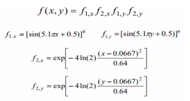
STALAGMITE FUNCTION CODE :

function [f] = stalagmite(input_vector)

x = input_vector(1);
y = input_vector(2);

term1 = (sin(5.1*pi*x + 0.5))^6;
term2 = exp(-4*log(2)*((x-0.0667)^2)/(0.64));
term3 = (sin(5.1*pi*y + 0.5))^6;
term4 = exp(-4*log(2)*(y-0.0667)^2/(0.64));
f = -1*(term1*term2*term3*term4); %negative sign is to invert the function, thus finding the maxima%
end

“ga” function syntax:

x= ga(fun,nvars) finds a local unconstrained minimum, x, to the objective function, fun. nvars is the dimension (number of design variables) of fun.
x= ga(fun,nvars,A,b) finds a local minimum x to fun, subject to the linear inequalities A*x ≤ b. ga evaluates the matrix product A*x as if x is transposed (A*x').
x= ga(fun,nvars,A,b,Aeq,beq) finds a local minimum x to fun, subject to the linear equalities Aeq*x = beq and A*x ≤ b. (Set A=[] and b=[] if no linear inequalities exist.) ga evaluates the matrix product Aeq*x as if x is transposed (Aeq*x').
x= ga(fun,nvars,A,b,Aeq,beq,lb,ub) defines a set of lower and upper bounds on the design variables, x, so that a solution is found in the range lb ≤ x ≤ ub. (Set Aeq=[] and beq=[] if no linear equalities exist.)
x= ga(fun,nvars,A,b,Aeq,beq,lb,ub,nonlcon) subjects the minimization to the constraints defined in nonlcon. The function nonlcon accepts x and returns vectors C and Ceq, representing the nonlinear inequalities and equalities respectively. ga minimizes the fun such that C(x) ≤ 0 and Ceq(x) = 0. (Set lb=[] and ub=[] if no bounds exist.)
x= ga(fun,nvars,A,b,Aeq,beq,lb,ub,nonlcon,options) minimizes with the default optimization parameters replaced by values in options. (Set nonlcon=[] if no nonlinear constraints exist.) Create options using optimoptions.

fun – objective function :

Objective function, specified as a function handle or function name. Write the objective function to accept a row vector of length ‘nvars’ and return a scalar value.

When the 'UseVectorized' option is true, write fun to accept a pop-by-nvars matrix, where pop is the current population size. In this case, fun returns a vector the same length as pop containing the fitness function values. Ensure that fun does not assume any particular size for pop, since ga can pass a single member of a population even in a vectorized calculation.

Example: fun = @(x)(x-[4,2]).^2

Data Types: char | function_handle | string

Nvars – Number of variables:

Number of variables, specified as a positive integer. The solver passes row vectors of length nvars to fun.

Example: 4

Data Types: double

A, b – Linear inequality constraints:

Linear inequality constraints, specified as a real matrix or a real vector respectively . A is an M-by-nvars matrix, where M is the number of inequalities. b is an M-element vector related to the A matrix. If you pass b as a row vector, solvers internally convert b to the column vector b(:)

A,b encodes the M linear inequalities

A*x <= b,

where x is the column vector of nvars variables x(:), b is a column vector with M elements and A is a matrix of size M-by-N.

For example, to specify

x₁ + 2x₂ ≤ 10
3x₁ + 4x₂ ≤ 20
5x₁ + 6x₂ ≤ 30,

give these constraints:

A = [1,2;3,4;5,6];

b = [10;20;30];

Example: To specify that the control variables sum to 1 or less, give the constraints A = ones(1,N) and b = 1.

Data Types: double

Aeq, beq – Linear equality constraints:

Linear equality constraints, specified as a real matrix or a real vector respectively. Aeq is an Me-by-nvars matrix, where Me is the number of equalities. beq is an Me-element vector related to the Aeq matrix. If you pass beq as a row vector, solvers internally convert beq to the column vector beq(:).

Aeq,beq encodes the Me linear equalities

Aeq*x = beq,

where x is the column vector of N variables x(:), Aeq is a matrix of size Meq-by-N and beq is a column vector with Me elements.

For example, to specify

x₁ + 2x₂ + 3x₃ = 10
2x₁ + 4x₂ + x₃ = 20,

give these constraints:

Aeq = [1,2,3;2,4,1];

beq = [10;20];

Example: To specify that the control variables sum to 1, give the constraints Aeq = ones(1,N) and beq = 1.

Data Types: double

lb – Lower Bounds:

Lower bounds, specified as a real vector or array of doubles. lb represents the lower bounds element-wise in lb ≤ x ≤ ub.

Internally, ga converts an array lb to the vector lb(:).

Default value = [ ]

Example: lb = [0;-Inf;4] means x(1) ≥ 0, x(3) ≥ 4.

Data Types: double

up – Upper Bounds:

Upper bounds, specified as a real vector or array of doubles. ub represents the upper bounds element-wise in lb ≤ x ≤ ub.

Internally, ga converts an array ub to the vector ub(:).

Default value = [ ]

Example: ub = [Inf;4;10] means x(2) ≤ 4, x(3) ≤ 10.

Data Types: double

nonlcon – non linear constraints:

Nonlinear constraints, specified as a function handle or function name. nonlcon is a function that accepts a vector or array x and returns two arrays, c(x) and ceq(x).

c(x) is the array of nonlinear inequality constraints at x. ga attempts to satisfy

c(x) <= 0

for all entries of c.

ceq(x) is the array of nonlinear equality constraints at x. ga attempts to satisfy

ceq(x) = 0

for all entries of ceq.

For example,

x = ga(@myfun,4,A,b,Aeq,beq,lb,ub,@mycon)

where mycon is a MATLAB^® function such as

function [c,ceq] = mycon(x)

c = ... % Compute nonlinear inequalities at x.

ceq = ... % Compute nonlinear equalities at x.

options – Optimisation Options:

Optimization options, specified as the output of optimoptions or a structure.

optimoptions hides the options listed in italics.

Values in {}denote the default value.
{}*represents the default when there are linear constraints, and for MutationFcn also when there are bounds.
I*indicates that ga handles options for integer constraints differently; this notation does not apply to gamultiobj.
NMindicates that the option does not apply to gamultiobj.

CASE I: STATISTICAL BEHAVIOUR WITHOUT BOUNDS

Code:

%Study-1: Statistical Behaviour without bounds

clear all
close all
clc

%Defining our search space and iterations
x = linspace(0,0.6,150);
y = linspace(0,0.6,150);
num_cases = 100     %number of iterations


%Creating a 2Dimensional mesh
[x, y] = meshgrid(x, y);

%Evaluating the stalagmite function
for i = 1:length(x)
    for j = 1:length(y)
        input_vector(1) = x(i,j);
        input_vector(2) = y(i,j);
        f(i,j) = stalagmite(input_vector);
    end
end


tic
for i= 1:num_cases                              %finding value for each iteration
    [inputs,fopt(i)] = ga(@stalagmite,2);      %calling genetic algorithm function
    xopt(i) = inputs(1);
    yopt(i) = inputs(2);
end
case1_time = toc

subplot(2,1,1);     %creating a subplot to have 2 plots in same figure
hold on 
surf(x,y,f);      %inverting again to plot actual stalagmite
shading interp;     %shading on
plot3(xopt,yopt,fopt,'marker','o','markersize',5,'markerfacecolor','r');
xlabel('x-axis');
ylabel('y-axis');
title('unbounded inputs');
subplot(2,1,2);
plot(fopt);
xlabel('Iterations');
ylabel('Function minimum');

Output:

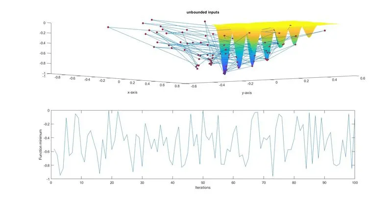
Conclusion: The optimum value keeps changing and is randomised with no scope of converging. Hence, this approach is wrong.

CASE II: STATISTICAL BEHAVIOUR WITH BOUNDS

Code:

%Study-2: Statistical Behaviour with bounds

clear all
close all
clc

%Defining our search space and iterations
x = linspace(0,0.6,150);
y = linspace(0,0.6,150);
num_cases = 100     %number of iterations


%Creating a 2Dimensional mesh
[x, y] = meshgrid(x, y);

%Evaluating the stalagmite function
for i = 1:length(x)
    for j = 1:length(y)
        input_vector(1) = x(i,j);
        input_vector(2) = y(i,j);
        f(i,j) = stalagmite(input_vector);
    end
end

tic
for i = 1:num_cases
    [inputs,fopt(i)] = ga(@stalagmite,2,[],[],[],[],[0;0],[0.6;0.6]);    %setting bounds from 0 to 0.6
    xopt(i) = inputs(1);
    yopt(i) = inputs(2);
end
case2_time = toc
subplot(2,1,1);     %creating a subplot to have 2 plots in same figure
hold on 
surf(x,y,f);      %inverting again to plot actual stalagmite
shading interp;     %shading on
plot3(xopt,yopt,fopt,'marker','o','markersize',5,'markerfacecolor','r');
xlabel('x-axis');
ylabel('y-axis');
title('Bounded Inputs');
subplot(2,1,2);
plot(fopt);
xlabel('iterations');
ylabel('function minimum');

Output:

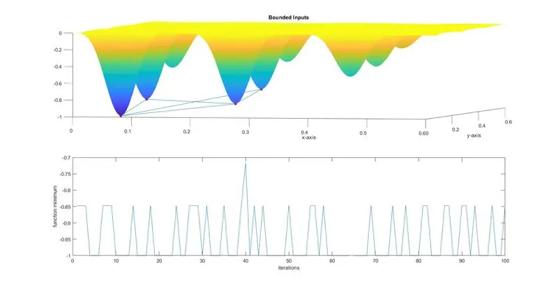
Conclusion: The optimum value keeps switching between two values but is structured. Hence, this approach is right but can be improved further.

CASE III: STATISTICAL BEHAVIOUR WITH BOUNDS AND LARGER POPULATION

Code:

%Study-3: Statistical Behaviour with bounds and larger population

clear all
close all
clc

%Defining our search space and iterations
x = linspace(0,0.6,150);
y = linspace(0,0.6,150);
num_cases = 100     %number of iterations


%Creating a 2Dimensional mesh
[x, y] = meshgrid(x, y);

%Evaluating the stalagmite function
for i = 1:length(x)
    for j = 1:length(y)
        input_vector(1) = x(i,j);
        input_vector(2) = y(i,j);
        f(i,j) = stalagmite(input_vector);
    end
end

tic
options = optimoptions('ga');
options = optimoptions(options,'PopulationSize',170);   %changing the population size to 170

% Input Arguments
% fun = @stalagmite
% nvar = 2
% A = []
% b = []
% Aeq = []
% beq = []
% lb = [0;0]
% ub = [0.1;0.1]
% nonlcon = []
% Intcon = []
% '[]' represents null value, whereas '{}' represents default value

for i = 1:num_cases
    [inputs,fopt(i)] = ga(@stalagmite,2,[],[],[],[],[0;0],[0.1;0.1],[],[],options);    %setting bounds from 0 to 0.1
    xopt(i) = inputs(1);
    yopt(i) = inputs(2);
end
case3_time = toc
subplot(2,1,1);     %creating a subplot to have 2 plots in same figure
hold on 
surf(x,y,-f);      %inverting again to plot actual stalagmite
shading interp;     %shading on
plot3(xopt,yopt,-fopt,'marker','o','markersize',5,'markerfacecolor','r');
xlabel('x-axis');
ylabel('y-axis');
title('bounded inputs with bigger population');
subplot(2,1,2);
plot(-fopt);
xlabel('iterations');
ylabel('function maximum');

Output:

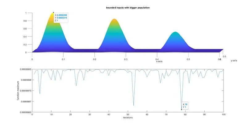
Conclusion: The optimum value is almost constant with negligible error. Hence, this approach is right and gives the correct answer. Thus, the maximum value of the stalagmite function under our search space is approximately equal to '1'.

CODE EXPLANATION:

Clearing workspace and defining our search space and number of iterations.
Creating a 2D mesh of search space.
Evaluating the stalagmite function for surface plot.
For each iteration, using ga function to calculate the maximum value.
Plotting the stalagmite function and maximum values.

ERRORS:

Basic syntax errors were encountered which were resolved immediately.

REFERENCES:

Genetic Algorithm - Finding the global maximum of a Stalagmite Function.

Ship work like this
in your own course.

Talk to a career counsellor

Ship work like thisin your own course.

Talk to a career counsellor

Ship work like this
in your own course.