Week 4 - Genetic Algorithm
AIM:
To perform the concept of Genetic algorithm and write a code of case study of Statistical behvaiour of (ga).
OBJECTIVE:
Write a code in MATLAB to optimise the stalagmite function and find the global maxima of the function.
Clearly explain the concept of genetic algorithm in your own words and also explain the syntax for Genetic Algorithm (ga) in MATLAB
THEORY:
Genetic algorthim:
A genetic algorithm is a search heuristic that is inspired by Charles Darwin’s theory of natural evolution. This algorithm reflects the process of natural selection
where the fittest individuals are selected for reproduction in order to produce offspring of the next generation.
Genetic algorithm solves smooth or nonsmooth optimization problems with any types of constraints, including integer constraints.
It is a stochastic, population-based algorithm that searches randomly by mutation and crossover among population members.
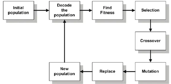
BLOCK DIAGRAM OF GENETRIC ALGORITHM
Notion of Natural Selection:
The process of natural selection starts with the selection of fittest individuals from a population.They produce offspring which inherit the characteristics
of the parents and will be added to the next generation. If parents have better fitness, their offspring will be better than parents and have a better
chance at surviving. This process keeps on iterating and at the end, a generation with the fittest individuals will be found.
This notion can be applied for a search problem. We consider a set of solutions for a problem and select the set of best ones out of them.
Five phases are considered in a genetic algorithm.
1.Initial population
2.Fitness function
3.Selection
4.Crossover
5.Mutation
Initial population:
The process begins with a set of individuals which is called a Population. Each individual is a solution to the problem you want to solve.
An individual is characterized by a set of parameters (variables) known as Genes. Genes are joined into a string to form a Chromosome (solution).
In a genetic algorithm, the set of genes of an individual is represented using a string, in terms of an alphabet. Usually, binary values are used (string of 1s and 0s).
We say that we encode the genes in a chromosome.
Fitness Function:
The fitness function determines how fit an individual is (the ability of an individual to compete with other individuals). It gives a fitness score to each individual.
The probability that an individual will be selected for reproduction is based on its fitness score.
Selection:
The idea of selection phase is to select the fittest individuals and let them pass their genes to the next generation.
Two pairs of individuals (parents) are selected based on their fitness scores. Individuals with high fitness have more chance to be selected for reproduction.
Cross over:
Crossover is the most significant phase in a genetic algorithm. For each pair of parents to be mated, a crossover point is chosen at random from within the genes.
Offspring are created by exchanging the genes of parents among themselves until the crossover point is reached.
The new offspring are added to the population.
Mutation:
In certain new offspring formed, some of their genes can be subjected to a mutation with a low random probability.
This implies that some of the bits in the bit string can be flipped.
Stalagmite function:
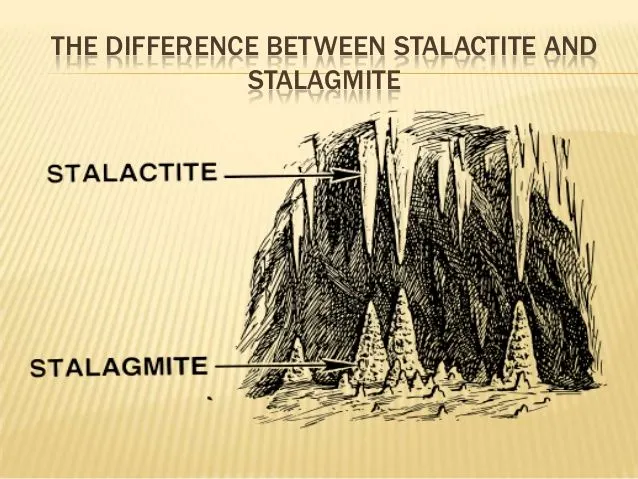
STALACTITE: Hanged from the celling points. Pointed ends.
STALAGMITE: Rise from the floor. Round or flatted ends.
Here the function is named as get_stalagmite, only the minimum value is obtained by using ga. Inorder to obtain maximum value
a slight change is made ie the -f(x,y) is taken. on the contest we get the maximum value.
SYNTAX ga IN MATLAB:
x = ga(fun,nvars)
x = ga(fun,nvars,A,b)
x = ga(fun,nvars,A,b,Aeq,beq)
x = ga(fun,nvars,A,b,Aeq,beq,lb,ub)
x = ga(fun,nvars,A,b,Aeq,beq,lb,ub,nonlcon)
x = ga(fun,nvars,A,b,Aeq,beq,lb,ub,nonlcon,options)
x = ga(fun,nvars,A,b,[],[],lb,ub,nonlcon,IntCon)
x = ga(fun,nvars,A,b,[],[],lb,ub,nonlcon,IntCon,options)`
x = ga(problem)
[x,fval] = ga(___)
[x,fval,exitflag,output] = ga(___)
[x,fval,exitflag,output,population,scores] = ga(___)
where,
fun - function name
nvars - Number of variables
A - Linear inequality constraints as real matrix
B - Linear inequality constraints as real vector
Aeq - Linear equality constraints as real matrix
Beq - Linear equality constraints as real vector
lb - Lower Boundary
ub - upper Boundary
nonlcon - Non linear constraints
option - Creating optimisation option using 'optimoptions'
MAIN CODE FUNCTION(get_Stalagmite):
%Program of get_stalagmite Function

function [f] = get_stalagmite(input_vector)

%Inputs
x = input_vector(1);
y = input_vector(2);

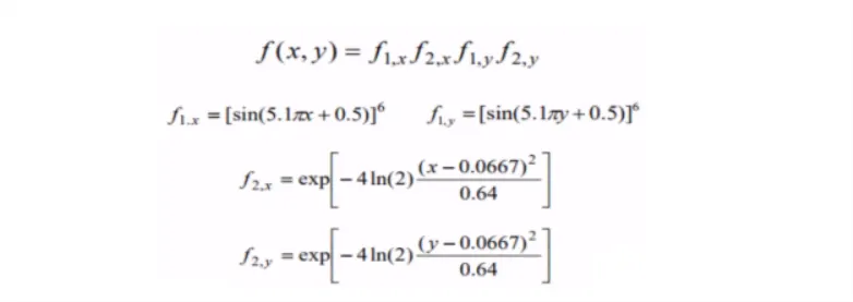
%Solution of the function f(x,y) = (f_1,x)*(f_2,x)*(f_1,y)*(f_1,y)

%sf1 = f1,x
%sf2 = f1,y
%sf3 = f2,x
%sf4 = f2,y


sf1 = (sin((5.1*pi*x )+ 0.5))^6;
sf2 = (sin((5.1*pi*y) + 0.5))^6;
sf3 = exp(-4*log(2)*((x-0.0667)^2)/0.64);
sf4 = exp(-4*log(2)*((y-0.0667)^2)/0.64);

f = -(sf1*sf2*sf3*sf4);

end
MAIN CODE:
close all
clear all
clc

x=linspace(0,0.6,150);
y=linspace(0,0.6,150);

num_case = 50 %total no of iterations

%calculating stalagmite function and equality to vector f

[xx,yy]= meshgrid(x,y);

for i=1:length(xx)
   for j=1:length(yy)
       input_vector(1)=xx(i,j);
        input_vector(2)=yy(i,j);
    f(i,j)=get_stalagmite(input_vector);
   end
end

%study1-statistical behaviour with unbounded inputs
tic
for i=1:num_case
  [inputs,fopt(i)]=ga(@get_stalagmite,2);
    xopt(i)=inputs(1);
    yopt(i)=inputs(2);

end
  study_time= toc
  figure(1)
  subplot(2,1,1)
  hold on
  surfc(x,y,f)
  shading interp
  plot3(xopt,yopt,fopt,'marker','o','markersize',5,'markerfacecolor','r')
  title('unbounded inputs')
  subplot(2,1,2)
  plot(fopt)
  xlabel('interations')
  ylabel('function minimium')

%study2-statistical behaviour with upper and lower bounds

for i=1:num_case
    [inputs,fopt(i)]=ga(@get_stalagmite,2,[],[],[],[],[0;0],[1;1]);
     xopt(i)=inputs(1);
     yopt(i)=inputs(2);
end

study_time2 = toc
 figure(2)
  subplot(2,1,1)
  hold on
  surfc(x,y,f)
  shading interp
  plot3(xopt,yopt,fopt,'marker','o','markersize',5,'markerfacecolor','r')
  title('bounded inputs')
  subplot(2,1,2)
  plot(fopt)
  xlabel('interations')
  ylabel('function minimium')

%study3 increasing GA interations
options= optimoptions('ga');
options= optimoptions(options,'populationsize',150);

tic
for i=1:num_case
   [inputs,fopt(i)]=ga(@get_stalagmite,2,[],[],[],[],[0;0],[1;1],[],[],options);
    xopt(i)=inputs(1);
    yopt(i)=inputs(2);
end

study_time3 = toc
 figure(3)
  subplot(2,1,1)
  hold on
  surfc(x,y,f)
  shading interp
  plot3(xopt,yopt,fopt,'marker','o','markersize',5,'markerfacecolor','r')
  title('bounded inputs with modified population size')
  subplot(2,1,2)
  plot(fopt)
  xlabel('interations')
  ylabel('function minimium')
Step wise explantion of code:
1.First of all using clear all , close all and clc commands for making sure only the program variables are used in the code and all other get erased by using this command.
2.The search space of ga is defined using linspace command, from this command we can understand that the x and y array value should be in between (0,0.6,150)
values are used as search space.
3.The no. of iterations for ga is defined as (num_cases = 50)
4. using meshgrid command we can create a 2D plot with the arrary of x and y defined above
5.For loop is used to give inputs to( get_stalagmite function) inputs which means while running 50 iterations the value changes
6.First – Statistical behaviour with unbounded inputs : In this the optimum values for the inputs taken for each iterations with the help of a for loop
Study timers commands tic and toc commands are used
the ga syntax used first study (unbounded inputs)
x=ga(fun,nvars)
7. Plotting commands
8. Figure command is used for opening a figure window and subplot command is used to get multiple plot in one figure window.
Plot3 command is used for getting the surface as 3D
Then the title command is used for getting title for the plot also labelled
9. In second study, the same parameters are used only the difference is in using(the syntax of ga is upper and lower bounds) are used in second study.
the ga syntax used in second study (Upper & Lower Bounded Inputs )
x = ga(fun,nvars,A,b,Aeq,beq,lb,ub)
10.In third study the plotting commands are used as same above but the suntax of ga changed by using optimoptions and increased iterations/population size to 170.
the ga syntax used third study (Increases iterations/population size using OPtimoptions)
x = ga(fun,nvars,A,b,Aeq,beq,lb,ub,nonlcon,IntCon,options)
OUTPUT CASE 1:
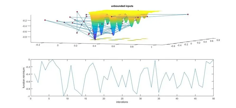
OUTPUT CASE 2:
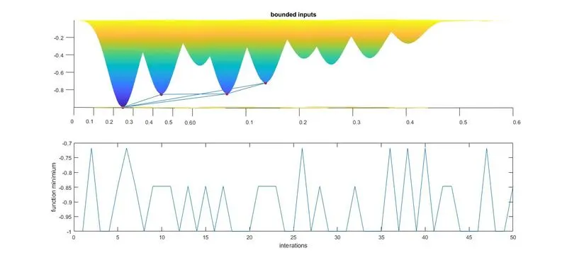
OUTPUT CASE 3:
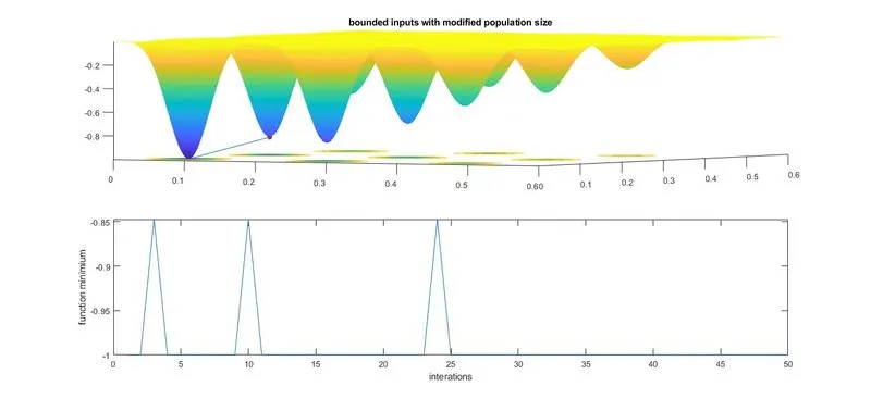
ERRORS:
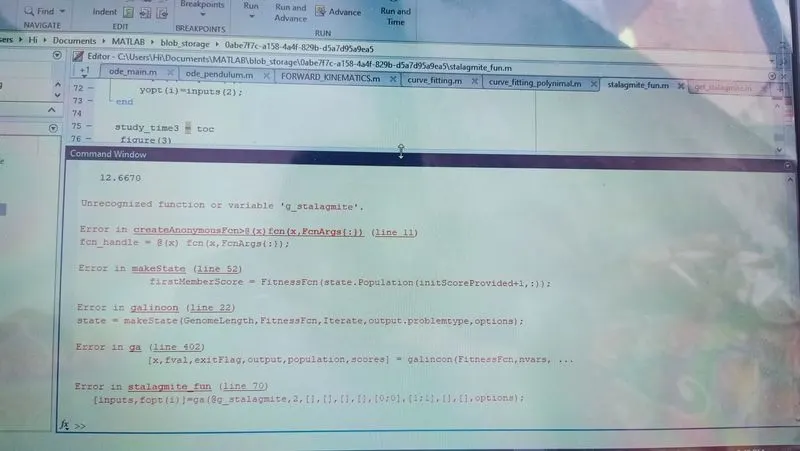
I was done error in syntax function code. its error was g_stalagmite (get_stalagmite).
so replace the synax code.the function is runing with out error.
WORKSPACE:
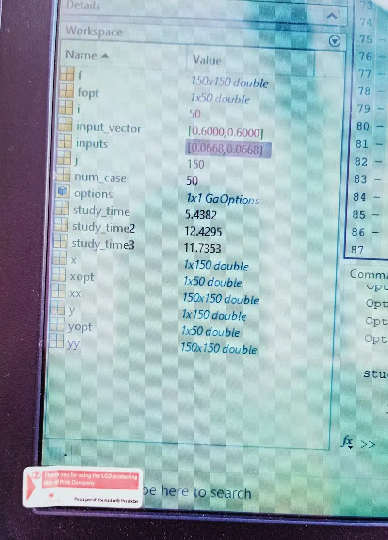
CONCULSION:
The concept of ga is studied and done 3 case studies on the statistical behaviour of the ga, in each case different syntax of ga is used
Study time 1 = 7.1392 sec , Study time 2 =18.3246 sec , Study time 3 = 23.5814 sec
when population size increases the precision in value of global maxima also increases also depends on syntax genetic algorithm(ga)
The max value obtained = 0.85.
REFERENCE:
https://in.mathworks.com/help/gads/constrained-minimization-using-ga.html