Project 2 - Rankine cycle Simulator
AIM:
To write a program ideal rankine cycle simulator using in matlab
OBJECTIVE:
To calculate the performance of a Steam turbine Engine.
To collect the inlet turbine pressure, outlet turbine pressure and boiler temperature.
Using the data calculate the state points of the rankine cycle. state points include enthalpy and entropy of system.
Then calculate the performace parameters of the given rankine cycle.
To plot the T-S and H-S diagram of a Rankine Cycle.
THEORY:
Rankine cycle:
The Rankine cycle is a model used to predict the performance of steam turbine systems.Rankine cycle consits of an operating fluid which
continuously gets evaporated and condensed in a close loop.
Components used:-
1. Boiler for generating steam at constant pressure
2. A turbine or engine in which steam will expand isentropically and work is done.
3. A condenser in which heat is removed from the exhaust steam and it is completely converted into water at constant pressure.
4.A pump which raises the pressure of liquid water to boiler pressure and pumps it in to the boiler for converting into steam.
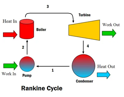
The simple Rankine cycle consists of 4 processes .
I’ll be using this numbered block diagram to make the explanation easier.
We’ll start with the water entering the boiler :
Process4−1: This is the process during which heat is added to the water to evaporate it (and even superheat it) . The heat addition takes place at constant pressure
Process 1−2: This is the process during which we get useful work from the cycle. In this process the steam expands in the turbine,exiting it at the condenser pressure.
This process is assumed to be isentropic .
Process 2−3: This is the process during which the (wet) steam exiting the turbine rejects heat (in the condenser which is simply a heat exchanger).
This process is essential so that all the steam is condensed to saturated liquid . This heat rejection takes place at constant pressure
Process 3−4: After all the steam becomes a saturated liquid , the water’s pressure is raised to the boiler pressure using the pump . This process is assumed to be isentropic
So now after discussing each process in detail , The cycle can be summarized as :
- Constant pressure heat addition
- Isentropic expansion
- Constant pressure heat rejection
- Isentropic compression
This is also the T-S diagram of the simple cycle which will be useful when you’re trying to visualize these processes and also when you move on to the improvements .
In general, the efficiency of a simple rankine cycle can be written as

Each of the next four equationsis derived from the energy and mass balance for a control volume. eth thermal defines the thermodynamic efficiency
of the cycle as the ratio of net power output to heat input. As the work required by the pump is often around 1% of the turbine work output, it can be simplified.




When dealing with the efficiencies of the turbines and pumps, an adjustment to the work terms must be made:


MATLAB CODE:
close all
clear all
clc

disp('RANKINE CYCLE');
disp('1-2 is Iscentropic Expansion in the Turbine');
disp('2-3 is Constant Pressure Heat rejection by the Condensor');
disp('3-4 is Iscentropic Expansion in the Pump');
disp('4-1 is Constant Pressure Heat addition to the Boiler');

%Inputs:
disp('INPUTS');
P1 = input('Enter the Pressure at turbine inlet(bar):');
T1 = input('Enter the Temperature at the Turbine inlet(degree C):');
P2 = input('Enter the Pressure at the Condensor(bar):');

%Using the XSteam functions,the enthalpy and entropy at various
%points can be calculated:

%Caluclating enthalpy(h) and entropy(s) at point 1:
h1 = XSteam('h_pT',P1,T1);
s1 = XSteam('s_pT',P1,T1);

%Caluclating pressure(P),enthalpy(h) and entropy(s) at point 2:

%Since Iscentropic Expansion:
s2=s1;

%For Iscentropic Expansion:
% wkt (T2/T1)=(P2/P1)^(1-(1/g))
g = 1.4;
power = 1-(1/g);

%Hence (T2/T1) = (P2/P1)^power:
T2 = T1*((P2/P1)^power);
h2 = XSteam('h_pT',P2,T2);

%Caluclating pressure(P),enthalpy(h) and entropy(s) at point 3:

%Since Constant Pressure Heat Removal:
P3 = P2;
T3 = T2;
h3 = XSteam('hL_T',T3);
s3 = XSteam('sL_T',T3);

%Caluclating pressure(P),enthalpy(h) and entropy(s) at point 4:

%Since Iscentropic Compression:
s4 = s3;

%Since Constant Pressure Process:
P4 = P1;

T4 = XSteam('T_ps',P4,s4);
h4 = XSteam('h_pT',P4,T4);
h41 = XSteam('hL_p',P4);
s41 = XSteam('sL_p',P4);
h42 = XSteam('hV_p',P4);
s42 = XSteam('sV_p',P4);
T41 = XSteam('T_hs',h41,s41);
T42 = XSteam('T_hs',h42,s42);

%Calculating the Entropy and Enthapy at the saturation curve:

Temp = linspace(0,500,600);

for i = 1:length(Temp)

sv(i) = XSteam('sV_T',Temp(i));
sl(i) = XSteam('sL_T',Temp(i));

hv(i) = XSteam('hV_T', Temp(i));
hl(i) = XSteam('hL_T', Temp(i));

end

%Calculating Net Work Output(W_net):

W_t = h1-h2;
W_p = h4-h3;
W_net = W_t-W_p;

%Calculating Back Work Ratio:
Bw_ratio = W_p/W_t;

%Calculating the Thermal efficiency:
Q_in = h1-h4;
eff_thermal = (W_net/Q_in)*100;

%Calculating Specific Steam Consumption:
% wkt 1J = 3600kg/s
SSC = 3600/W_net;

% Displaying Results in the command window:
disp('                       Results                       ');
P1 = P1;
T1 = T1;
P2 = P2;
disp('At stage point 1');
n1 = sprintf('P1 is %.3f bar',P1);
disp(n1);
n2 = sprintf('T1 is %.3f C',T1);
disp(n2);
n3 = sprintf('h1 is %.3f kJ/kg',h1);
disp(n3);
n4 = sprintf('s1 is %.3f kJ/kgK',s1);
disp(n4);
disp('At stage point 2');
n11 = sprintf('P2 is %.3f bar',P2);
disp(n11);
n21 = sprintf('T2 is %.3f C',T2);
disp(n21);
n31 = sprintf('h2 is %.3f kJ/kg',h2);
disp(n31);
n41 = sprintf('s2 is %.3f kJ/kgK',s2);
disp(n41);
disp('At stage point 3');
n12 = sprintf('P3 is %.3f bar',P3);
disp(n12);
n22 = sprintf('T3 is %.3f C',T3);
disp(n22);
n32 = sprintf('h3 is %.3f kJ/kg',h3);
disp(n32);
n42 = sprintf('s3 is %.3f kJ/kgK',s3);
disp(n42);
disp('At stage point 4');
n13 = sprintf('P4 is %.3f bar',P4);
disp(n13);
n23 = sprintf('T4 is %.3f C',T4);
disp(n23);
n33 = sprintf('h4 is %.3f kJ/kg',h4);
disp(n33);
n43 = sprintf('s4 is %.3f kJ/kgK',s4);
disp(n43);
n14 = sprintf('W_t is %.3f kJ/kg',W_t);
disp(n14);
n15 = sprintf('W_p is %.3f kJ/kg',W_p);
disp(n15);
n16 = sprintf('W_net is %.3f kJ/kg',W_net);
disp(n16);
n17 = sprintf('Eff_Thermal is %.2f Percent',eff_thermal);
disp(n17);
n18 = sprintf('SSC is %.2f kg/kWh',SSC);
disp(n18);

figure(1)
plot([s1 s2],[T1 T2],[s2 s3],[T2 T3],[s3 s4],[T3 T4],[s4 s41],[T4 T41],[s41 s42],[T41 T42],[s42 s1],[T42 T1],'marker','*','color','r')
hold on
plot(sv,Temp)
plot(sl,Temp)
title('T-S Diagram')
xlabel('Entropy-s(kJ/kgK');
ylabel('Temperature-T(K)');

figure(2)
plot([s1 s2],[h1 h2],[s2 s3],[h2 h3],[s3 s4],[h3 h4],[s4 s1],[h4 h1],'marker','*','color','r')
hold on
plot(sv,hv)
plot(sl,hl)
title('H-S Diagram')
xlabel('Entropy-s(kJ/kgK');
ylabel('Enthalpy-h(kJ/k)');
Procedure:
The following code does the following:
- Initially, it takes in values for the inlet, outlet conditions of turbine and boiler temperature
2. Then it calculates the entropy for second state point as expansion in turbine is isentropic.
values for entropies and other data in the code is exported fromthe XSteam.m file given.
3. using the obtained data entropy at third state point is known with which entropy at boiler inlet is also obtained as pump in an isentropic process
4. Similarly values for enthalpy is also found out.
5. using the appropriate formulas and the data generated the performance parameters of the rankine cycle is found out.
6. The required data as asked is printed as output.
7. For plotting of T-S diagram : isentropic process and constant pressure heat addition and rejection at latent heat temperature follow a straight line.
So, can be plotted with two end points
8. For constant pressure heat addition and rejection at sensible heat temperatures it follows the constant pressure line hence data is to be generated at each point.
This is done by making use of a for loop
9. Finally if the dryness fraction is grater than one at turbine outlet condition then heat rejection in condensor will initially follow the constant pressure
curve until it reaches the saturation vapour temperature. if less than one the steam is wet in condition.
OUTPUTS:
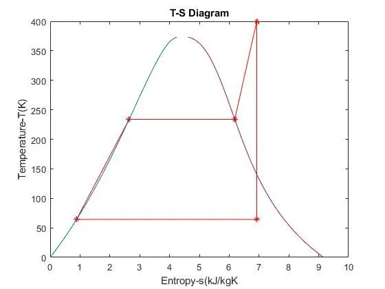
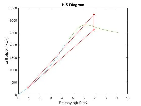
command window:
  RANKINE CYCLE
1-2 is Iscentropic Expansion in the Turbine
2-3 is Constant Pressure Heat rejection by the Condensor
3-4 is Iscentropic Expansion in the Pump
4-1 is Constant Pressure Heat addition to the Boiler
  INPUTS
Enter the Pressure at turbine inlet(bar):30
Enter the Temperature at the Turbine inlet(degree C):400
Enter the Pressure at the Condensor(bar):0.05

                       Results

At stage point 1
P1 is 30.000 bar
T1 is 400.000 C
h1 is 3231.571 kJ/kg
s1 is 6.923 kJ/kgK

At stage point 2
P2 is 0.050 bar
T2 is 64.314 C
h2 is 2620.455 kJ/kg
s2 is 6.923 kJ/kgK

At stage point 3
P3 is 0.050 bar
T3 is 64.314 C
h3 is 269.206 kJ/kg
s3 is 0.885 kJ/kgK

At stage point 4
P4 is 30.000 bar
T4 is 64.446 C
h4 is 272.229 kJ/kg
s4 is 0.885 kJ/kgK

W_t is 611.116 kJ/kg
W_p is 3.023 kJ/kg
W_net is 608.093 kJ/kg
Eff_Thermal is 20.55 Percent
SSC is 5.92 kg/kWh
Conclusion:
The performance of the Heat Engine was calculated and the following Observations were made:
Net Work = 608.093 kJ/kg
Thermal Efficiency = 20.55%
Back Work Ratio = 0.4%
The T-S and H-S performance curves of the Rankine Cycle were plotted.
Reference: