Challenge

Genetic Algorithm using MATLAB

SSaransh Dimri23 Dec 2020

Objective: -

Develop a code in MATLAB to optimize the stalagmite function and find the global maxima of the function. And to explain the concept of genetic algorithm and also the syntax for ga in MATLAB. And to plot the graphs for all 3 studies and for F maximum vs no. of iterations.

Principle: -

A genetic algorithm is a search heuristic that is inspired by Charles Darwin’s theory of natural evolution. This algorithm reflects the process of natural selection where the fittest individuals are selected for reproduction in order to produce offspring of the next generation

Solution Procedure: -

The process of natural selection starts with the selection of the fittest individuals from a population. They produce offspring which inherit the characteristics of the parents and will be added to the next generation. If parents have better fitness, their offspring will be better than parents and have a better chance of surviving. This process keeps on iterating and in the end, a generation with the fittest individuals will be found.

This notion can be applied to a search problem. We consider a set of solutions for a problem and select the set of best ones out of them.

Five phases are considered in a genetic algorithm.

Initial population
Fitness function
Selection
Crossover
Mutation

Genetic algorithms are randomized search algorithms that have been developed in an effort to imitate the mechanics of natural selection and natural genetics. Genetic algorithms operate on string structures, like biological structures, which are evolving in time according to the rule of survival of the fittest by using a randomized yet structured information exchange. Thus, in every generation, a new set of strings is created, using parts of the fittest members of the old set. The main characteristics of a genetic algorithm are as follows: -

The genetic algorithm works with the coding of the parameter set, not the parameters themselves.
The genetic algorithm initiates its search from a population of points, not a single point.
The genetic algorithm uses payoff information, not derivatives.
The genetic algorithm uses probabilistic transition rules, not deterministic ones

A genetic algorithm (GA) is a method for solving both constrained and unconstrained optimization problems based on a natural selection process that mimics biological evolution. The algorithm repeatedly modifies a population of individual solutions. At each step, the genetic algorithm randomly selects individuals from the current population and uses them as parents to produce the children for the next generation. Over successive generations, the population "evolves" toward an optimal solution.

You can apply the genetic algorithm to solve problems that are not well suited for standard optimization algorithms, including problems in which the objective function is discontinuous, nondifferentiable, stochastic, or highly nonlinear.

The genetic algorithm differs from a classical, derivative-based, optimization algorithm in two main ways, as summarized in the following table.

Classical Algorithm	Genetic Algorithm
Generates a single point at each iteration. The sequence of points approaches an optimal solution.	Generates a population of points at each iteration. The best point in the population approaches an optimal solution.
Selects the next point in the sequence by a deterministic computation.	Selects the next population by computation which uses random number generators.

Outline of the Genetic Algorithm: -

The following outline summarizes how the genetic algorithm works:

The algorithm begins by creating a random initial population.
The algorithm then creates a sequence of new populations. At each step, the algorithm uses the individuals in the current generation to create the next population. To create a new population, the algorithm performs the following steps:
1. Scales the raw fitness scores to convert them into a more usable range of values. These scaled values are called expectation values.
2. Selects members, called parents, based on their expectations.
3. Some of the individuals in the current population that have lower fitness are chosen as elite. These elite individuals are passed to the next population.
4. Produces children from their parents. Children are produced either by making random changes to a single parent mutation by combining the vector entries of a pair of parents crossover
5. Replaces the current population with the children to form the next generation.
Scores each member of the current population by computing its fitness value. These values are called raw fitness scores.
The algorithm stops when one of the stopping criteria is met.

Stalagmite Function: -

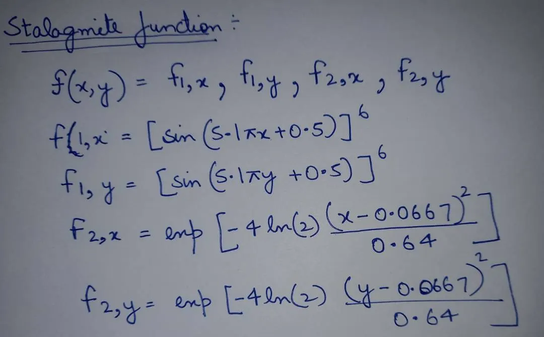
CODE for the stalagmite function: -

function[f] = stalagmite(input_vector)

%Intializing x and y input

x=input_vector(1);
y=input_vector(2);

%term X1 is equation for f1_x and term Y1 is equation for f1_y 
termX1 = (sin(5.1*pi*x +0.5))^6;
termY1 = (sin(5.1*pi*y + 0.5))^6;


%term X2 is the equation for f2_x and term Y2 is the equation for f2_y 

termX2 = exp(-4*log(2)*((x-0.0667)^2/0.64));
termY2 = exp(-4*log(2)*((y-0.0667)^2/0.64));


f = termX1*termY1*termX2*termY2;

end

Explanation of the above code: -

function[f] = stalagmite(input_vector) - function to perform the task of stalagmite function
%Intializing x and y input - comments to make a program user friendly
x=input_vector(1); -to initialize the first column
y=input_vector(2); - to initialize the second column
%term X1 is equation for f1_x and term Y1 is equation for f1_y - comments
termX1 = (sin(5.1*pi*x +0.5))^6; - initializing the term according to the equation
termY1 = (sin(5.1*pi*y + 0.5))^6; - initializing the term according to the equation
%%term X2 is equation for f2_x and term Y2 is equation for f2_y
termX2 = exp(-4*log(2)*((x-0.0667)^2/0.64));- initializing the term according to the equation
termY2 = exp(-4*log(2)*((y-0.0667)^2/0.64));- initializing the term according to the equation
f = termX1*termY1*termX2*termY2; - calculating the value according tho the stalagmite function
end - to terminate the function

CODE for the Genetic Algorithm:-

%Program for a Genetic Algorithim
clear all
close all
clc

%Defining our search space

x= linspace(0,0.6,150);
y= linspace(0,0.6,150);

%Creating a 2Dimensional mesh
[xx,yy] = meshgrid(x,y);

%Evaluating the stalagmite function

for i = 1:length(xx)
    for j = 1:length(yy)
        input_vector(1)=xx(i,j);
        input_vector(2)=yy(i,j);
        f(i,j)= stalagmite(input_vector);
    end
end

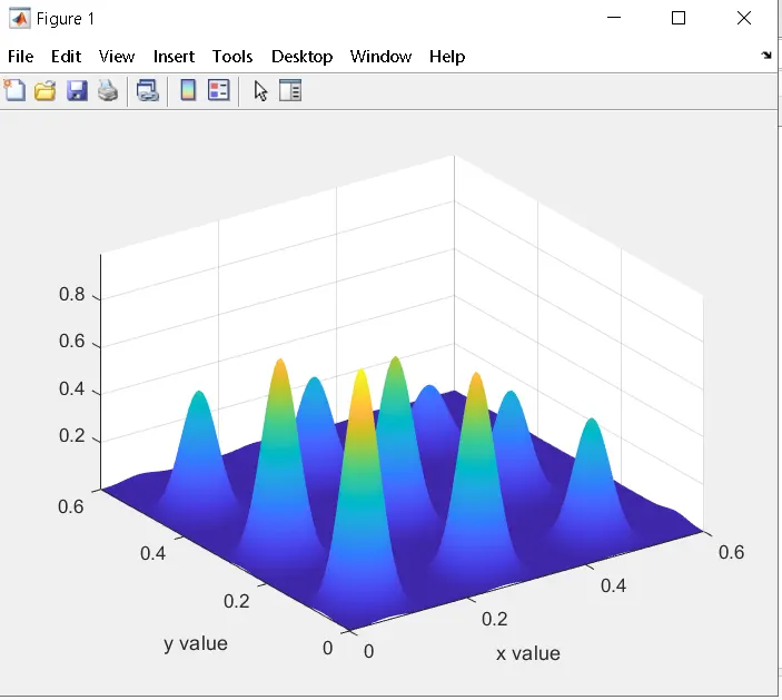
surfc(xx,yy,f)
xlabel('x value')
ylabel('y value')

shading interp

[inputs , fval] = ga(@stalagmite,2)

Explanation of the above code: -

%Program for a Genetic Algorithm - comments
clear all -to clear all the workspace variables
close all - to close all the output window
clc - to clear the command window

%Defining our search space

x= linspace(0,0.6,150); - linspace is used to generate 150 values between 0 and 0.6
y= linspace(0,0.6,150); - linspace is used to generate 150 values between 0 and 0.6
%Creating a 2Dimensional mesh
[xx,yy] = meshgrid(x,y); - used to create a dimensional array

%Evaluating the stalagmite function - comments

for i = 1:length(xx) - for execution of the statements in loop till length(xx)
for j = 1:length(yy) - for execution of the statements in loop till length(yy)
input_vector(1)=xx(i,j); - initializing the array rows and column
input_vector(2)=yy(i,j); -initializing the array rows and column
f(i,j)= stalagmite(input_vector); calling the stalgamite function to get the value by passing input vector
end - to terminate the for loop
surfc(xx,yy,f) - it is used to generate a surface plot
xlabel('x value') - for labelling the x value
ylabel('y value') - for labelling the y value
shading interp - to remove gridlines on the plot
[inputs , fval] = ga(@stalagmite,2) - it is the syntax for genetic algorithim

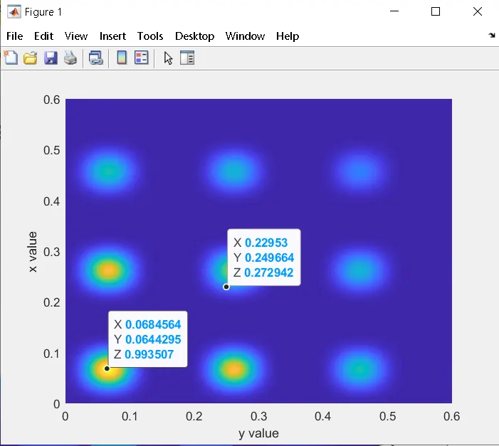
Output of the above code: -

Syntax for Genetic Algorithim: -

x = ga(fun,nvars)
x = ga(fun,nvars,A,b)
x = ga(fun,nvars,A,b,Aeq,beq)
x = ga(fun,nvars,A,b,Aeq,beq,lb,ub)
x = ga(fun,nvars,A,b,Aeq,beq,lb,ub,nonlcon)
x = ga(fun,nvars,A,b,Aeq,beq,lb,ub,nonlcon,options)
x = ga(fun,nvars,A,b,[],[],lb,ub,nonlcon,IntCon)
x = ga(fun,nvars,A,b,[],[],lb,ub,nonlcon,IntCon,options)
x = ga(problem)
[x,fval] = ga(___)
[x,fval,exitflag,output] = ga(___)
[x,fval,exitflag,output,population,scores] = ga(___)

Description of the above Syntax: -

x = ga(fun,nvars,A,b) finds a local minimum x to fun, subject to the linear inequalities A*x<=b ga evaluates the matrix product A*x as if x is transposed (A*x')

x = ga(fun,nvars,A,b,Aeq,beq) finds a local minimum x to fun , subject to the linear equalities Aeq*x=beq and A*x<=b(Set A=[] and b=[] if no linear inequalities exist.) ga evaluates the matrix product Aeq*x as if x is transposed (Aeq*x')

x = ga(fun,nvars,A,b,Aeq,beq,lb,ub)defines a set of lower and upper bounds on the design variables,x, so that a solution is found in the rangelb<=x<=ub(Set A=[] and b=[] if no linear inequalities exist.)

x = ga(fun,nvars,A,b,Aeq,beq,lb,ub,nonlcon) subjects the minimization to the constraints defined in nonclon The function nonclon accepts x and returns vectors C and Ceq, representing the nonlinear inequalities and equalities respectively.ga minimizes the fun such that C(x)<=0 and Ceq(x)<0

x = ga(fun,nvars,A,b,Aeq,beq,lb,ub,nonlcon,Intcon,options)minimizes with the default optimization parameters replaced by values in options (Set nonlcon[] if no nonlinear constraints exist.) Create options using optimoptions

x = ga(fun,nvars,A,b,Aeq,beq,lb,ub,nonlcon,Intcon,options) requires that the variables listed in Intcon take integer values.

x = ga(problem)finds the minimum for problem,a structure described in problem.[x,fval] = ga(___)for any previous input arguments, also returns fval, the value of the fitness function at x

[x,fval,exitflag,output ] = ga(___)also returns exitflag an integer identifying the reason the algorithm terminated,output a structure that contains output from each generation and other information about the performance of the algorithm

[x,fval,exitflag,output,population,scores ] = ga(___)also returns a matrix population , whose rows are the final population, and a vector scores, the scores of the final population.

CODE for Study 1: -

%Program for a Genetic Algorithim
clear all
close all
clc

%Defining our search space

x= linspace(0,0.6,150);
y= linspace(0,0.6,150);
num_case = 50;
%Creating a 2Dimensional mesh
[xx,yy] = meshgrid(x,y);

%Evaluating the stalagmite function

for i = 1:length(xx)
    for j = 1:length(yy)
        input_vector(1)=xx(i,j);
        input_vector(2)=yy(i,j);
        f(i,j)= stalagmite(input_vector);
    end
end

%Study 1-Statistical behaviour
tic
for i = 1:num_case
    [inputs , fopt(i)] = ga(@stalagmite,2);
    xopt(i) = inputs(1);
    yopt(i) = inputs(2);
end
study1_time = toc

figure(1)
subplot(2,1,1)
hold on
surfc(x,y,-f)
xlabel('x value')
ylabel('y value')
shading interp

plot3(xopt,yopt,-fopt,'marker','o','markersize',5,'markerfacecolor','r')
title('Unbound inputs')
subplot(2,1,2)
plot(-fopt)
xlabel('Iterations')
ylabel('Function minimum')

Explanation of the above code: -

%Program for a Genetic Algorithim - comments

clear all -to clear all the workspace variables
close all - to close all the output window
clc - to clear the command window
x= linspace(0,0.6,150); - linspace is used to generate 150 values between 0 and 0.6
y= linspace(0,0.6,150); - linspace is used to generate 150 values between 0 and 0.6
num_case = 50 - to run the genetic algorithm 50 times
%Creating a 2Dimensional mesh
[xx,yy] = meshgrid(x,y); - used to create a dimensional array

%Evaluating the stalagmite function - comments

for i = 1:length(xx) - for execution of the statements in loop till length(xx)
for j = 1:length(yy) - for execution of the statements in loop till length(yy)
input_vector(1)=xx(i,j); - initializing the array rows and column
input_vector(2)=yy(i,j); -initializing the array rows and column
f(i,j)= stalagmite(input_vector); calling the stalgamite function to get the value by passing input vector
end - to terminate the for loop
surfc(xx,yy,f) - it is used to generate a surface plot
xlabel('x value') - for labelling the x value
ylabel('y value') - for labelling the y value
shading interp - to remove gridlines on the plot

%Study 1-Statistical behaviour

tic - command use to check how much does it take to complete
for i = 1:num_case - for execution of the statements in loop till 50 times
[inputs , fopt(i)] = ga(@stalagmite,2); - syntax for gentic algorithim
xopt(i) = inputs(1); - to initialize the x optimum value
yopt(i) = inputs(2); - to initialize the y optimum value
end - to terminate the for loop
study1_time = toc - command use to check how much does it take to complete
figure(2) - to generate a figure window
subplot(2,1,1) - to have multiple plor inside the same figure window
hold on - to change the hold state to on
surfc(x,y,f) - to generate the surface plot
xlabel('x value') - labelling the x axis
ylabel('y value') - labeling the y axis
shading interp - to remove the gridlines on the graph
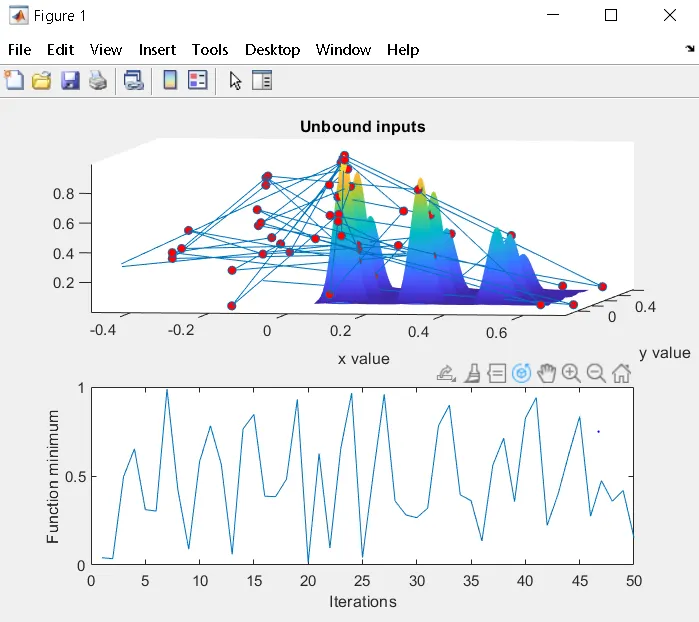
plot3(xopt,yopt,fopt,'marker','o','markersize',5,'markerfacecolor','r') - to plot optimum value that ga predict over the 50 studies
title('Unbound inputs') - to give title topmthe plot

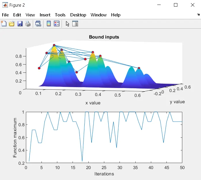
Output for the Unbounded inputs :-

CODE for study 2: -

%Program for a Genetic Algorithim
clear all
close all
clc

%Defining our search space

x= linspace(0,0.6,150);
y= linspace(0,0.6,150);
num_case = 50;
%Creating a 2Dimensional mesh
[xx,yy] = meshgrid(x,y);

%Evaluating the stalagmite function

for i = 1:length(xx)
    for j = 1:length(yy)
        input_vector(1)=xx(i,j);
        input_vector(2)=yy(i,j);
        f(i,j)= stalagmite(input_vector);
    end
end

tic
%Study 2 for the optimization

for i = 1:num_case
    [inputs , fopt(i)] = ga(@stalagmite,2,[],[],[],[],[0:0],[0.5:0.5]);
    xopt(i) = inputs(1);
    yopt(i) = inputs(2);
end
study2_time = toc

figure(2)
subplot(2,1,1)
hold on
surfc(x,y,-f)
xlabel('x value')
ylabel('y value')
shading interp

plot3(xopt,yopt,-fopt,'marker','o','markersize',5,'markerfacecolor','r')
title('Bound inputs')
subplot(2,1,2)
plot(-fopt)
xlabel('Iterations')
ylabel('Function maximum')

Explanation of the above code: -

%Study 2 - Optimization using Bounded input

tic - command use to check how much does it take to complete
for i = 1:num_case - for execution of the statements in loop till 50 times
[inputs , fopt(i)] = ga(@stalagmite,2,[],[],[],[],[0:0],[0.5:0.5]); - syntax for gentic algorithim
xopt(i) = inputs(1); - to initialize the x optimum value
yopt(i) = inputs(2); - to initialize the y optimum value
end - to terminate the for loop
study2_time = toc - command use to check how much does it take to complete
figure(2) - to generate a figure window
subplot(2,1,1) - to have multiple plor inside the same figure window
hold on - to change the hold state to on
surfc(x,y,f) - to generate the surface plot
xlabel('x value') - labelling the x axis
ylabel('y value') - labeling the y axis
shading interp - to remove the gridlines on the graph
plot3(xopt,yopt,fopt,'marker','o','markersize',5,'markerfacecolor','r') - to plot optimum value that ga predict over the 50 studies
title('Unbound inputs') - to give title to the plot

Output for the bounded inputs :-

CODE for study 3: -

%Program for a Genetic Algorithm
clear all
close all
clc

%Defining our search space

x= linspace(0,0.6,150);
y= linspace(0,0.6,150);
num_case = 50;
%Creating a 2Dimensional mesh
[xx,yy] = meshgrid(x,y);

%Evaluating the stalagmite function

for i = 1:length(xx)
    for j = 1:length(yy)
        input_vector(1)=xx(i,j);
        input_vector(2)=yy(i,j);
        f(i,j)= stalagmite(input_vector);
    end
end

options = optimoptions('ga')
options = optimoptions(options,'populationsize',360);
tic
%Study 2 for the optimization

for i = 1:num_case
    [inputs , fopt(i)] = ga(@stalagmite,2,[],[],[],[],[0:0],[0.5:0.5],[],[],options);
    xopt(i) = inputs(1);
    yopt(i) = inputs(2);
end
study2_time = toc

figure(2)
subplot(2,1,1)
hold on
surfc(x,y,-f)
xlabel('x value')
ylabel('y value')
shading interp

plot3(xopt,yopt,-fopt,'marker','o','markersize',5,'markerfacecolor','r')
title('Bound inputs')
subplot(2,1,2)
plot(-fopt)
xlabel('Iterations')
ylabel('Function maximum')

Explanation of the above code: -

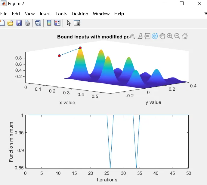
%Study 3 - Optimization using Bounded input with population size

options = optimoptions('ga') - to set the population size minimize with non default options
options = optimoptions(options,'populationsize',360);
tic - command use to check how much does it take to complete
for i = 1:num_case - for execution of the statements in loop till 50 times
[inputs , fopt(i)] = ga(@stalagmite,2,[],[],[],[],[0:0],[1:1],[],[],options); - syntax for gentic algorithim
xopt(i) = inputs(1); - to initialize the x optimum value
yopt(i) = inputs(2); - to initialize the y optimum value
end - to terminate the for loop
study2_time = toc - command use to check how much does it take to complete
figure(2) - to generate a figure window
subplot(2,1,1) - to have multiple plor inside the same figure window
hold on - to change the hold state to on
surfc(x,y,f) - to generate the surface plot
xlabel('x value') - labelling the x axis
ylabel('y value') - labeling the y axis
shading interp - to remove the gridlines on the graph
plot3(xopt,yopt,fopt,'marker','o','markersize',5,'markerfacecolor','r') - to plot optimum value that ga predict over the 50 studies
title('Unbound inputs') - to give title to the plot

Output for the bounded inputs with modified population size :-

CODE for the genetic algorithm: -

%Program for a Genetic Algorithim
clear all
close all
clc

%Defining our search space

x= linspace(0,0.6,150);
y= linspace(0,0.6,150);
num_case = 50;
%Creating a 2Dimensional mesh
[xx,yy] = meshgrid(x,y);

%Evaluating the stalagmite function

for i = 1:length(xx)
    for j = 1:length(yy)
        input_vector(1)=xx(i,j);
        input_vector(2)=yy(i,j);
        f(i,j)= stalagmite(input_vector);
    end
end

%Study 1-Statistical behaviour
tic
for i = 1:num_case
    [inputs , fopt(i)] = ga(@stalagmite,2);
    xopt(i) = inputs(1);
    yopt(i) = inputs(2);
end
study1_time = toc

figure(1)
subplot(2,1,1)
hold on
surfc(x,y,f)
xlabel('x value')
ylabel('y value')
shading interp

plot3(xopt,yopt,fopt,'marker','o','markersize',5,'markerfacecolor','r')
title('Unbound inputs')
subplot(2,1,2)
plot(fopt)
xlabel('Iterations')
ylabel('Function minimum')


tic
%Study 2 for the optimization

for i = 1:num_case
    [inputs , fopt(i)] = ga(@stalagmite,2,[],[],[],[],[0:0],[1:1]);
    xopt(i) = inputs(1);
    yopt(i) = inputs(2);
end
study2_time = toc

figure(2)
subplot(2,1,1)
hold on
surfc(x,y,f)
xlabel('x value')
ylabel('y value')
shading interp

plot3(xopt,yopt,fopt,'marker','o','markersize',5,'markerfacecolor','r')
title('Bound inputs')
subplot(2,1,2)
plot(fopt)
xlabel('Iterations')
ylabel('Function minimum')


options = optimoptions(@ga)
options = optimoptions(options,'populationsize',170);
tic
%Study 3 for the optimization

for i = 1:num_case
    [inputs , fopt(i)] = ga(@stalagmite,2,[],[],[],[],[0:0],[1:1],[],[],options);
    xopt(i) = inputs(1);
    yopt(i) = inputs(2);
end
study3_time = toc

figure(3)
subplot(2,1,1)
hold on
surfc(x,y,f)
xlabel('x value')
ylabel('y value')
shading interp

plot3(xopt,yopt,fopt,'marker','o','markersize',5,'markerfacecolor','r')
title('Bound inputs')
subplot(2,1,2)
plot(fopt)
xlabel('Iterations')
ylabel('Function minimum')

Explanation of the above code: -

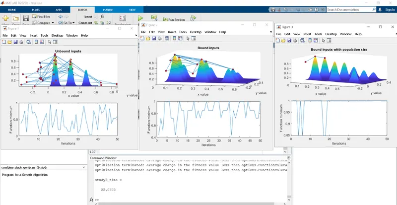
Above code is the combination all the codes explained before individually for the different stages of genetic algorithim

Output for the Genetic Algorithim:-

Errors faced during developing the code: -

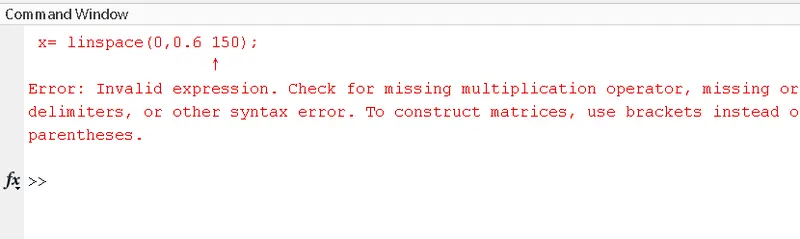
error raised for an Invalid expression.

On debugging it was found out that a (,) was missing in the linspace method variables

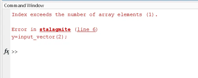
Error due to exceeding of number of array elements

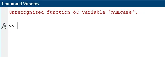
An error was found because of an Unrecognized function or variable 'numcase'.

It was because the 'num_case was not a variable used it 'numcase' which was used

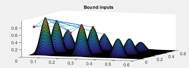
Was getting grid lines in the graph

On debugging it was found shading intrep was missing

Conclusion: -

Study time for 1st study was 2.55 sec
Study time for 2nd study was 3.44 sec
Study time for 3rd study was 21.65 sec
The stalagmite equation multiplied by -1 to generate a downward stalagmite
F = -f so that the minimum value of f is the maximum value for F and vice versa

References: -

Genetic Algorithm using MATLAB

Ship work like this
in your own course.

Talk to a career counsellor

Ship work like thisin your own course.

Talk to a career counsellor

Ship work like this
in your own course.