Week 4 - Genetic Algorithm

Problem Statement:

• Write a code in MATLAB to optimize the stalagmite function and find the global maxima of the function.
• Clearly explain the concept of genetic algorithm in your own words and also explain the syntax for ga in MATLAB in your report.
• Make sure that your code gives the same output, even if it is made to run several times.
• Plot graphs for all 3 studies and for F maximum vs no. of iterations. Title and axes labels are a must, legends could be shown if necessary.

Aim: To write a code to optimize the stalagmite function and find its global maxima of the function.

Description:

What is Optimization? Optimization is a technique or process of selection of best choices from a set of variables. It refers to finding the best value of outputs for a set of Inputs. The best value changes from

problem to problem.

Components:

1.Decision Variables
2. Objective Function
3.Constraints

Decision Variables:

The optimization technique starts by Identifying the decision variables. And then relating them with the objective function, constraints. Variables can be continuous, semi-continuous, discrete, and can be bounded or unbounded.

Objective Function:

Function with respect to which the decision variables are optimized. They can be also continuous or semi-continuous.
If there are NO objective functions only the presence of constraints leads to a feasible problem.

Constraints:

Two Types

1.Equality constraints
2. Inequality Constraints.

Classification of Optimization Problems:

1.Linear Programming
2.Non Linear Programming
3.Integer Linear Programming
4.Mixed Integer Linear Programming
5. Mixed Integer Linear Programming

Classification Of Optimization Techniques:

(i)Mathematical Programming Techniques(Based on Geometric Properties Of the Problem.)

1.Simplex algorithm, Interior point algorithm.
2.Steepest Decent, Newton's Method, Quasi-Newton
3. Branch & Bound, Cutting Planes

(ii) Metaheuristic Techniques

1.Genetic Algorithm
2.Particle Swarm Optimization
3.Differential Evolution
4.Teaching Learning Based Optimization
5.Artificial Bee Colony

(iii) Other Techniques

1. Nelder Mead/simplex Search
2. Fibonacci Method
3.Golden Section Method
4 Hooke Jeeve's Pattern Search Method

optimization problems:

1.Travelling salesman
2.Knapsack problem
3.Map colouring (feasibility problem) feasibility problems are a subset of optimization problems but the reverse is not true.
4.sudoku (NO objective only constraints are present)

Applications:

1.Design of aircraft and aerospace structures for minimum cost
2.Design of electrical components like motors, generators and transformers
3.Design of pumps, turbines, heat exchangers for maximum efficiency
4.Determining the trajectories of space vehicles.
5.Production planning, scheduling and controlling

Genetic Algorithm:

The Genetic Algorithm is developed by Darwin's principle of Evolution. It is a search based optimization technique based on the principle of natural evolution. It is used to find optimal or local optimal solutions.

Basic Terminology:

Population: Population is a set of all solutions, or which is a search space for an optimal solution.

chromosome: A chromosome is a solution to a problem.

Gene: Each element in a chromosome is known as Gene.

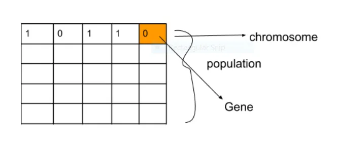
Basic Structure Of a GA: Initially we start with a population which is a set of solutions problems. Two parents are selected based on the fitness value of Individual solution and crossover and mutation technique

are performed to generate a new chromosome which is known as offsprings. These offsprings are added to the population. And the process continues till it generates the best optimal solution out of a set of

solutions.

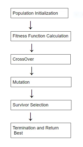
The most important part of the Genetic Algorithm is to deciding the representation we will use to represent our solutions.

It can be done in mainly three types:

1.Binary Representation.

2.Real Valued Representation.

3. Integer Representation.

4. Permutation Representation.

Population Initialization: The population is a set of Individual set of solutions. It is defined as a set of chromosomes. The diversity of the population should be maintained, the population should be large

because it will slow down the GA process.

Population Initialization can be done in two types 1.Random Initialization

2. Heuristic Initialization.

Fitness Function: The fitness function is defined as a function which takes an Individual solution to the problem as a

input and produces as output and considers how good the Individual solution is?

1.A fitness function should be so fast to compute.

2. It must measure how fit a given solution is.

Parent Selection: Parent selection is a process of selecting Individuals i.e Parents which mate together to produce offsprings for the next generation. It is a crucial step in GA because it will affect the convergence

of the solution. Parents are solution vectors from which the new set of solution set or next-generation are created, the new chromosomes are known as offsprings. Offspring are generated through mating by a

selection of good solution sets or by variation(crossover and mutation).

Parent Selection can be done mainly by

1.Fitness Proportionate Selection: In this, every Individual has the probability to become a parent which is proportional to their fitness value.so, every Individual has a very high chance of becoming a parent and

propagating their features to the next generation.

2. Roulette wheel selection: In Roulette wheel selection, a wheel is divided into segments based on their fitness value. A fixed point is chosen on the circumference of the circle. The part of the circle that comes in front of the fixed point is chosen as a parent. The second parent is chosen in the same way.

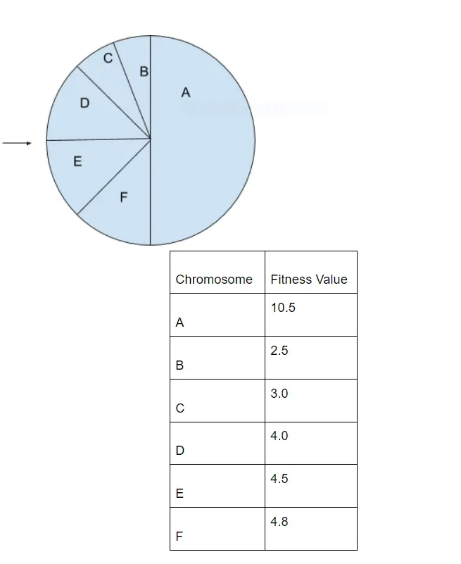
3.Stochastic Universal Sampling: It is similar to the Roulette Wheel Selection, Instead of the single fixed point we have two fixed points. And the selection of two parents is done in one single spin.

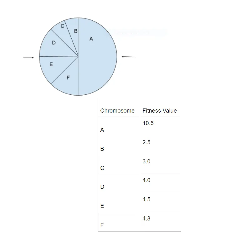
CrossOver: In the crossover, more than one parent is selected and offsprings are produced using the parent's genetic features.

CrossOver can be done by

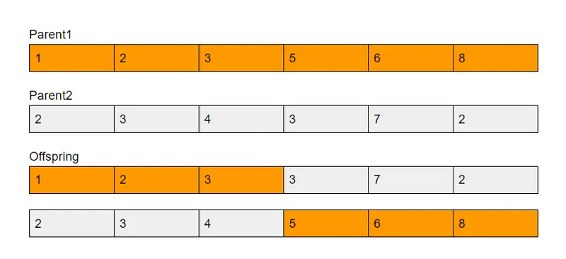
1.One Point CrossOver: In this random crossover point is selected and tails of two parents are swapped.

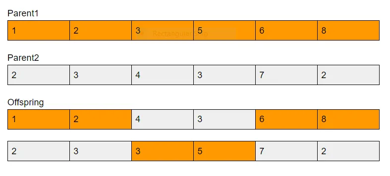
2.Multi Point CrossOver: In this multi crossover point are selected and tails are swapped to generate offsprings.

3.Arithmetic Representation: This is commonly works with Integer representation by taking a weighted average of two parents.

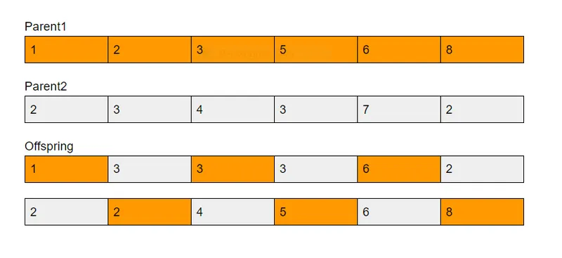
4.Uniform CrossOver: In this, we don't split the parent into segments rather we consider each gene, we can even bias gene to rather flip or not.

Mutation: mutation is defined as a small random tweak to the chromosome to maintain the diversity in the genetic population. It is Introduced two maintain diversity in genetic population.

Mutation can be done by 1.Bit Flip Mutation.

2.Random Resetting

3.Swap Mutation.

4.Scramble Mutation.

5. Inversion Mutation.

Survivor Selection: Survivor selection is a crucial step in which we decide whether the solution is to retain(to be kept in the next generation) or kicked out of the population. It should be noted that fitter

An individual should be retained by keeping diversity in the population. some GA employs Elitism that means the fittest Individual must be propagated to the next generations. The retaining of the Individual can

be done by 1.Age Based Selection

2.Fitness Based Selection.

Termination Conditions: It determines whether the Ga program run will end. It is observed that the GA progresses very fast with better solutions in very few solutions. In later stages, we will use a terminal

condition to stop the run and obtain the optimal solution.

commonly used termination conditions:1.when there is no improvement in 'n' number of Iteration.

2. when the solution reaches a predefined value

3. When we reach a certain no. of generations.

GA Working: GA in MatLab works as follows:

1. The algorithm begins by creating a random initial population.
2. The algorithm scores or measures the fitness function value of each Individual.
3. Selects Individuals, called parents, based on their fitness value.
4. These parents are used to generate new offsprings by crossover and mutation process.
5. The parent member with high fitness values are retained and parents with low value are kicked off from the population.
6. The new offsprings are added to the current population to form new children.
7. The algorithm runs until reaches stopping criteria.

'ga' Syntax: In Matlab, ga is used to calculate a minimum of a function, following are the syntaxes

used for 'ga' in Matlab.

1. x = ga(fun,nvars)[This finds a local unconstrained minimum x,to the objective function,fun.nvars is the dimension of fun.]
2. x = ga(fun,nvars,A,b)[This finds a local minimum x to fun,subject to the linear inequalities A *x <=b.ga evaluates the matrix product A*x as if x is transposed (A*x')]
3. x =ga(fun,nvars,A,b,Aeq.beq)[This finds a local minimum x to fun,subjected to the linear inequalities Aeq*x = be and A*x<=b.ga evaluates the matrix product A*x as if x is transposed (A*x')]
4. x = ga(fun,nvars,A,b,Aeq,beq,lb,ub)[This defines a set of lower and upper bounds on design variable x so that a solution is find in the range lb<=x<=ub.]
5. x = ga(fun,nvars,A,b,Aeq,beql,ubnonlcon)[This subjects to the minimumization to the constrained in the nonlcon.The fun nonlcon accepts x nd returns vectors C ,Ceq,representing the nonlinear inequalities and equalitiesrespectively.ga minimizes the fun such that C(x)<=0 and Ceq(X)=0(set lb = [] and ub = [] if no bounds exist)
6. X = ga (fun,nvars,A,b,Aeq,beq,lb,ub,nonlcon,options)[This subjects to the minimumization to the constrained in the nonlcon.The fun nonlcon accepts x nd returns vectors C ,Ceq,representing the nonlinear inequalities and equalitiesrespectively.ga minimizes the fun such that C(x)<=0 and Ceq(X)=0](set lb = [] and ub = [] if no bounds exist)
7. x = ga(fun,nvars,A,b,[],[],lb,ub,nonlcon,Intcon) or x = ga(fun,nvars,A,b,[],[],lb,ub,noncon,Intcon,options)[This finds the minimum for a problem, where problem is a structure.]
8. x= ga(problem)[This finds the minimum fo problem where problem is a structure.]
9. [x,fval]=ga(_)[for any previous input arguments, also returns faval,the value of the fitness function at x]
10. [x,favl,exitflag,output]=ga(_)[This alsoreturns exitflag,an integer identifying the reason the algorithm terminated ,and output , a structure that contains output from each generation and other information about the performance of the algorithm]
11. [x,fval,exitflag,output,population,scores]=ga(__)[This also returns a matrix population,whose rows are the final population,and a vector scores,the scores of the final population.]

Input Arguments:

1. fun = objective function.
2. nvars = Numberof variables
3. A = linear inequality constraints
4. b = linear equality constraints
5. Aeq = linear equality constraints
6. beq = linear equality constraints
7. lb = lower bounds
8. ub = upper bounds
9. nonlcon = nonlinear constraints
10. options = optimization options
11. Intcon = Integer variables
12. Problem = Problem description

Output Arguments:

1. x = solution.
2. fval = objective function value at solution
3. exitflag = Reason ga stopped
4. output = Information about the optimization process.

Stopping conditions for the algorithm:

1. Number of Generations: The algorithm stops when the algorithm reaches a certain number of generations.
2. Fitness limit: The algorithm stops when the fitness value for the best point in the current population is less than or equal to fitness limit
3. Time limit: The algorithm stops when it reaches a certain time in seconds.

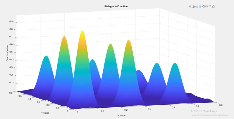
Stalagmite Function: The following equations are used in Matlab to define Stalagmite function.

`f(x,y) = f_1,_x f_2,_x f_1,_yf_2,_y`

where

`f_1,_x = [sin(5.1pix +0.5)]^6`

`f_2,_x = exp[-4ln(2)(x-0.0667)^2/0.64]`

`f_1,_y = [sin(5.1piy + 0.5)]^6`

`f_2,_y = exp[-4ln(2)(y-0.0667)^2/0.64]`

step by step procedure:

1. Intially a function is created which is stalagmite function and which is called using the function name in GA.
2. The algorithm starts with clearing and closing all the workspace, command window
3. The search space is defined using linspace command.
4. Evaluate the stalagmite function, which was created Initially.
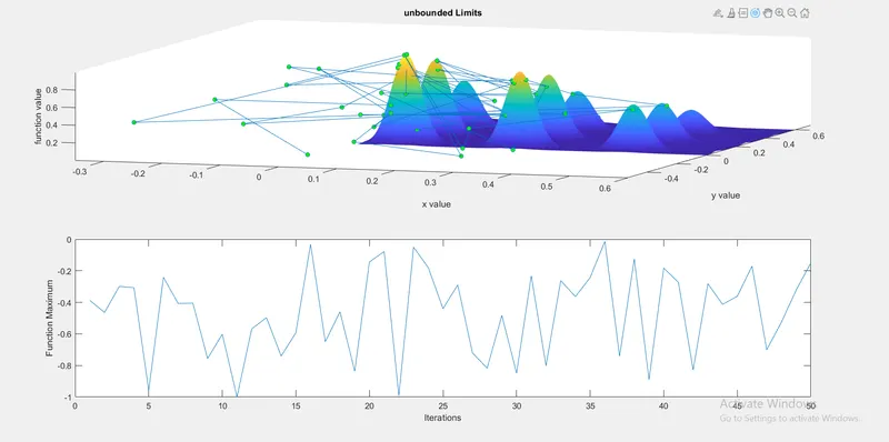
5. study1 is conducted without any bounded limits.
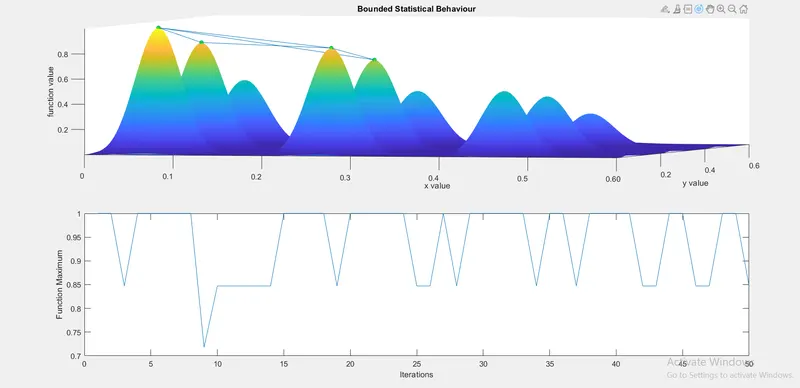
6. study2 is conducted with lower and upper bounds.
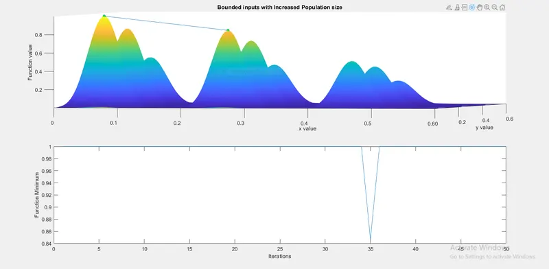
7. study3 is conducted with a function optimoptions to optimize the GA function.
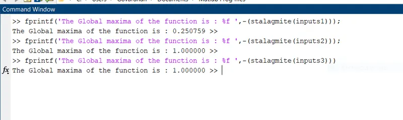
8. print all output using fprintf command.

Matlab code for the stalagmite function:

%%Define Function f is output, the function name is stalagmite.

function [f]= stalagmite(input_vector)
% Generating Input variables x,y
x = input_vector(1);
 y  = input_vector(2);
 
% Defining f1x and f1y function.
f1x = (sin(5.1*pi*x + 0.5))^6;
f1y = [sin(5.1*pi*y + 0.5)]^6;

% Defining f2x and f2y function.
f2x = exp(-4*log(2)*(((x-0.0667).^2)/0.64));
f2y = exp(-4*log(2)*((y-0.0667).^2)/0.64);

% Defining output function 'f'
f = (f1x*f1y*f2x*f2y);


end

Matlab code of Genetic Algorithm for stalagmite function

% Matlab code of Genetic Algorithm for stalagmite function

% Clear all workspace
% clear all command window.
% clear all plots

clear all
close all
clc


%% Defining our search space

x = linspace(0,0.6,150);
y = linspace(0,0.6,150);

% Defining the number of Iterations.
num_cases = 50;

% Generating 2D array

[xx,yy]= meshgrid(x,y);

for i = 1:length(xx)
    for j = 1:length(yy)
        input_vector(1) = xx(i,j);
        input_vector(2) = yy(i,j);
        % Defining the stalagmite function 
        f(i,j) = stalagmite(input_vector);
    end
end
figure(1)

% Defining the 3-D surface and determined by the range of x,y, z-axis
surfc(xx,yy,-f)

% Shading is a colour shading mode, controls the colour shading of surface
shading interp % for a smoother plot

% Defining the x,y,z labels
xlabel('x value')
ylabel('y value')
zlabel('Function Value')
title('Stalagmite Function')



% study1 Unbounded  statistical Behavior

% starts a stopwatch timer.
tic

for i = 1:num_cases 
    % passing ga function
    %[x , fval ]= ga(fun,nvars)
    % nvars = number of variables
    % fun = objective function
    [inputs1,fopt1(i)] = ga(@stalagmite,2);
    xopt1(i) = inputs1(1);
    yopt1(i) = inputs1(2);
end

% toc reads the stopwatch timer,tic and toc functions measure elapsed time.

study1_time = toc; 

figure(2)
% subplot creates the axis in tiled positions.
subplot(2,1,1)
hold on

surfc(xx,yy,-f)% Defining the 3-D surface and determined by the range of x,y,z axis
shading interp% Shading is a color shading mode , controls the color shading of surface
plot3(xopt1,yopt1,-fopt1,'marker','o','markersize',5,'markerfacecolor','g')

% Defining the x,y,z labels
title('unbounded inputs')
xlabel('x value')
ylabel('y value')
zlabel('function value')

% subplot creates the axis in tiled positions.
subplot(2,1,2)
plot(fopt1)

% Defining the x,y,z labels
xlabel('Iterations')
ylabel('Function Maximum')

% starts a stopwatch timer.
tic

% study2 with upper and lower bounds 

for i = 1:num_cases
     % passing ga function
    %[x , fval ]= ga(fun,nvars,A,b,[],[],lb,ub)
    % nvars = number of variables
    % fun = objective function
    [inputs2,fopt2(i)] = ga(@stalagmite,2,[],[],[],[],[0;0],[0.6;0.6]);
    xopt2(i) = inputs2(1);
    yopt2(i) = inputs2(2);
end

% toc reads the stopwatch timer,tic and toc functions measure elapsed time.

study2_time = toc

figure(3)
% subplot creates the axis in tiled positions.
subplot(2,1,1)
hold on

% Defining the 3-D surface and determined by the range of x,y, z-axis
surfc(xx,yy,-f)

% Shading is a colour shading mode, controls the colour shading of surface
shading interp% for a smoother plot

plot3(xopt2,yopt2,-fopt2,'marker','o','markersize',5,'markerfacecolor','g')

% Defining the x,y,z labels
xlabel('x value')
ylabel ('y value')
zlabel('function value')
title('Bounded Statistical Behaviour')

subplot(2,1,2)% subplot creates the axis in tiled positions.
plot(-fopt2)

% Defining the x,y,z labels
xlabel('Iterations')
ylabel('Function Maximum')

% study3 Increasing population size for a statistical behaviour

options = optimoptions(@ga);% By optimoptions we create options to optimize 'ga'
options = optimoptions(@ga,'populationsize',200)

% starts a stopwatch timer.
tic
for i = 1:num_cases
    % passing ga function
    %[x , fval ]= ga(fun,nvars,A,b,[],[],lb,ub,nonlcon,Intcon,options)
    % nvars = number of variables
    % fun = objective function
    [inputs3,fopt3(i)] = ga(@stalagmite,2,[],[],[],[],[0;0],[0.6;0.6],[],[],options);
    xopt3(i) = inputs3(1);
    yopt3(i) = inputs3(2);
end

% toc reads the stopwatch timer,tic and toc functions measure elapsed time.
study3_time = toc;

figure(4)
% subplot creates the axis in tiled positions.
subplot(2,1,1)
hold on

% Defining the 3-D surface and determined by the range of x,y, z-axis
surfc(x,y,-f)

% Shading is a colour shading mode, controls the colour shading of surface
shading interp% for a smoother plot

plot3(xopt3,yopt3,-fopt3,'marker','o','markersize',5,'markerfacecolor','g')

% Defining the x,y,z labels
title('Bounded inputs with Increased Population size')
xlabel('x value')
ylabel('y value')
zlabel('Function value')

subplot(2,1,2)% subplot creates the axis in tiled positions.
plot(-fopt3)

% Defining the x,y,z labels
xlabel('Iterations')
ylabel('Function Minimum')

%consolidated results

fprintf('study1:- Unbounded Statistical Behavior')
fprintf('The time taken for the study 1 is %f ',study1_time)
fprintf('The coodinates of x and y for the global maxima of the function is: %f,%f ',inputs1(1),inputs1(2))
fprintf('The Global maxima of the function is : %f ',-(stalagmite(inputs1)));



fprintf('study2:- Bounded Statistical Behavior')
fprintf('The time taken for the study 2 is %f ',study2_time)
fprintf('The coodinates of x and y for the global maxima of the function is: %f,%f ',inputs2(1),inputs2(2))
fprintf('The Global maxima of the function is : %f ',-(stalagmite(inputs2)));

fprintf('study3:- Icreasing population Statistical Behavior')
fprintf('The time taken for the study 3 is %f ',study3_time)
fprintf('The coodinates of x and y for the global maxima of the function is: %f,%f ',inputs3(1),inputs3(2))
fprintf('The Global maxima of the function is : %f ',-(stalagmite(inputs3)))











































    

output

Stalagmite function:

Study1 Output:

Study2 Output:

Study3 Output:

Command Window Output:

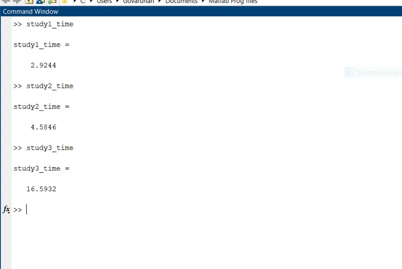
Time Taken For Each Study:

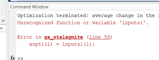
Errors:

1 I got errors while declaring the input vectors, Initially, I mentioned without column number.

Error Rectification:

Later on, by understanding the command window, I rectified my error.

References:

1.https://www.tutorialspoint.com/genetic_algorithms/index.htm

2.https://skill-lync.com/knowledgebase/genetic-algorithm-explained

3.https://www.youtube.com/watch?v=aJKuM4U-eYg

4.https://www.youtube.com/watch?v=LREPlWJmvAY