Matlab Programm To Solve A Otto Cycle

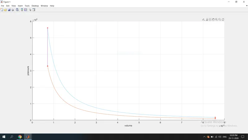
Aim : To create a pv diagram for OTTO Cycle using Matlab.

Description:The petrol Engine works on OTTO Cycle which is also know as constant volume cycle .

OTTO Cycle consists of four processes: 1. Reversible Adiabatic Compression.

2.Constant Volume Heat Addition.

3. Reversible Adiabatic Expansion.

4.Constant Volume Heat Rejection.

Formulas Used: compression ratio = cr = volume before compression/volume after compression.

swept volume = (pi/4)*bore diameter^2*stroke.

clearance volume = swept volume/(compression ratio - 1).

Engine Geometric Parameters: Bore Diameter= 0.1

stroke length = 0.1

compression ratio = 12

connecting rod = 0.15

Input Parameters: Gamma value = 1.4

Temperature at state 3 (t3)= 2300.

Pressure at state 1 (p1) = 101325.

Temperature at state 1 (t1) = 500

Explanation:

1. All state variables (p1,v1,T1;p2,v2,T2;p3,v3,T3;p4,v4,T4) are calculated by using the adiabatic equations i.e

pv^gamma = constant and Ideal Equation pv = n*r*T.

2.To know the change in volume between Top Dead Center (TDC)and Bottom Dead Center (BDC) by change in crank

angle ,will be calculated by using the following formula which is derived by Engine geometric parameters

v/Clearance volume = 1 + 0.5*(cr-1)*{(R+1-cosd(theta)-(R^2 - sind(theta)^2)^0.5}

Here R = con_rod/2

v is the volume covered by piston between TDC, BDC by change in the crank angle.

function[V] = piston_kinematics(bore,  stroke,con_rod,cr,start_crank,end_crank)
cr = 12;
a = stroke/2;
R = con_rod/a;

swept_vol = (pi/4)*bore^2*stroke;
clearance_volume = swept_vol/(cr-1);

theta = linspace(start_crank,end_crank,100)
term1 = 0.5*(cr-1);
term2 = R+1-cosd(theta);
term3 = (R^2 - sind(theta).^2).^0.5;
V = (1+term1*(term2-term3)).*clearance_volume

end

3.The 'v' is a function called in the otto cycle program.

clear all
close all
clc
%Inputs
gamma = 1.4;
t3 = 2300;

%state vaariables
p1 = 101325;
t1 = 500;

 %Engine Geometric Parameters.

 bore = 0.1;
 stroke = 0.1;
 con_rod =0.15;  
 cr = 12;

 %calculating the swept volume and clearance volume

 swept_vol = (pi/4)*bore^2*stroke;
 clearance_volume = swept_vol/(cr-1);
 v1 = swept_vol+ clearance_volume;
 v2 = clearance_volume;
 
 %state variables at point 2

 %p1*v1^gamma = p2*v2^gamma 
 %p2 = p1*(v2/v1)^gamma
 p2 = p1*(cr)^gamma
 
 %p1v1/t1 = p2v2/t2 | t2 = p2*v2*t1/p1*v1
  t2 = p2*v2*t1/(p1*v1);
  constant_c = p1*v1^gamma;
  v_compression = piston_kinematics(0.1,0.1,0.15,12,180,0)
 p_compression = constant_c./v_compression.^gamma;
  
  %state variables at point 3
  v3 = v2
  %p3v3/t3 = p2v2/t2 | p3 = p2*v2*t3/t2*v3
  p3 = p2*t3/t2
  constant_c = p3*v3^gamma;
  v_expansion = piston_kinematics(0.1,0.1,0.15,12,0,180)
 p_expansion = constant_c./v_expansion.^gamma 
  
  
  
  %state variables at point 4
  v4 = v1;
  %p4v4^gamma = p3v3^gamma |p4 = p3*(v3/v4)^gamma
  p4 = p3*(v3/v4)^gamma;
  
  
  figure(1)
  hold on  
  plot(v1,p1,'*','color','r')
  plot(v_compression,p_compression)
  plot(v2,p2,'*','color','r')
  plot([v2 v3],[p2 p3])
 plot(v3,p3,'*','color','r')
   plot(v_expansion,p_expansion)
  plot([v4 v1],[p4 p1])
  plot(v4,p4,'*','color','r')
xlabel('volume')
ylabel('pressure')
      
      
      grid on

4.The volume and pressure during compression process(i.e state2 to state3),during which crank angle changes

from 0 to 180 degrees is calculated as follows using

p*v^gamma = constant .

constant_c = p1*v1^gamma;
  v_compression = piston_kinematics(0.1,0.1,0.15,12,180,0)
 p_compression = constant_c./v_compression.^gamma;

5.The volume and pressure during expansion process (i.e state 4 to state 1),during which crank angle changes

from 0 to 180 degrees is calculated as follows using

p*v^gamma = constant .

constant_c = p3*v3^gamma;
  v_expansion = piston_kinematics(0.1,0.1,0.15,12,0,180)
 p_expansion = constant_c./v_expansion.^gamma

output: