Curve Fitting Using MATLAB.
Problem Statement:
1.Write code to fit a linear and cubic polynomial for the Cp data.
2.Plot the linear and cubic fit curves along with the raw data points. Title and axes labels are a must, legends could be shown if necessary.
3. Write a code to show splitwise method.
4. Explain the parameters used to measure the fitness characteristics for both the curves.
Aim: To know the mathematical behaviour of a data using Matlab.
Description:To know the mathematical behaviour of a data , we a concept know as curve fitting.
Curve Fitting : Curve Fitting is a process or a technique through which we can closely proximate the data
points.There are many curve fitting techniques 1.Interpolation Technique
2. Curve Fitting.
1.Interpolation Technique: In this technique the curve is drawn by point to point by Interpolating. It can be used when
the data follows a pattern or not in a cluster.
2.Curve Fitting: In this technique we equations to closely proximate the actual data points.In general polynomial
functions of 'n'th order are used . n = 1,2,3.....etc
The linear polynomial function is of y = ax + b .
y = is a dependent variable on 'x'.
second order polynomial function is of y = ax^2+bx+c .
Third order polynomial function y = ax^3 + bx^2 + cx + d.
Evaluating Goodness of a fit: The Goodness of a fit evaluates wheather the polynomial function used as a curve fit is good , or we will go for the higher order polynomial function which Interpolates more number
of data points.
There are four ways to check the Goodness of a fit :
1.The sum of squares due to error.
2. R - square.
3. Adjusted R - square.
4. Root Mean Squared Error.
1. The sum of squares due to error : Let us consider a polynomial function y = f(x), and the data
points are (x1,y1) , (x2,y2) , (x3,y3)......(xn,yn).
The error between the data point 'y' and the corresponding value of y at f(x) where
x = 1,2,3....n. is given by
Error = [Y - value of function y = f(X)] where Y = y1,y2,y3.....yn. X = x1,x2,x3..xn.
SSE(sum of squares) = `sum_(i = 1)^n (y_i - bary)^2` i = 1,2,3....n
Types of sum of squares :
1. Total sum of squares
SST = ∑i=1n(yi-y¯)2">n∑i=1(yi−¯y)2∑i=1n(yi-y¯)2
2. Regression Sum of squares:
SSR = ∑i=1n(y^i-y¯)2">n∑i=1(ˆyi−¯y)2∑i=1n(y^i-y¯)2
3.Resdual sum of squares
SSE = ∑i=1n(yi-y^i)2">n∑i=1(yi−ˆyi)2∑i=1n(yi-y^i)2
R - Square: It is a technique which defines the proporation of variance for a dependent variable by a Independent
variable.It explains the variance of one variable with respect to the another variable.
R² = SSR / SST
SST = SSR + SSE
Adjusted R Square : It only measures the variance of Independent variables that explains the
dependent variable and eliminates the variables which are Insignificant.
`R^2 = 1-[((1-R^2)(n-1))/(n-k-1)]`
Root mean squared error(RMSE): Root mean squared error tells about how the residue is spread out or tells how the data is compact around the line.
`RMSE = (SSE)/sqrtn`
MATLAB CODE:
To calculate the goodness of a fit, a function have created to calculate the RMSE value.
RMSE is calculated by creating a function programm.
function [RMSE]= calculate_rmse(cp,predicted_cp)

%%calculate Error

Error = cp - predicted_cp;

%% Total no. of samples

n = length(cp);

%%calculate SSE value

SSE = 0;
SUM = 0;
for i = 1:n
    SSE = SSE + Error(i)^2;
    SUM = SUM + cp(i);
end

%%calculate mean of the data

mean = SUM/2;
%% calculate SSR

SSR = 0;
for j = 1 : length(predicted_cp);
    SSR = SSR+(predicted_cp(i)- mean)^2;
end


%%calculte SST

SST = SSR + SSE;

%%Calculate R^2


R_Square = SSR/SST;

%%Calculate RMSE


RMSE = (SSE/n)^1/2;

end
2.Programm Code:
%% Program for curve fitting using 'n'th order polynomial


%% clering workspace,command window,plots
clear all
close all
clc

% preparing the data

cp_data = load('data');
cp = cp_data(:,2);
temp = cp_data(:,1);


% Curve fit
co_effs = polyfit(temp,cp,1); % polyfit command is used to calculate the coeficients of polynomial.

predicted_cp =  polyval(co_effs,temp);% polyval function is used to evaluate
                      output(predicted cp) by taking Inputs(coefficients,temperature)


%%plotting original curve

subplot(3,3,1)% Breaks the figure window into m-by-n matrix of small axis and selects
                                    the pth axis for the current plot.
plot(temp,cp,'linewidth',3,'color','r')

hold on
%% compare original curve and predicted curve

plot(temp,predicted_cp,'linewidth',3,'color','g')
legend('original data','1st order curve','location','northwest')
title('First Order curve')
xlabel('temp [k]')
ylabel('Specific Heat [KJ/KMOL-K]')
grid on


%%curve fit using second order polynomial

co_effs2 = polyfit(temp,cp,2);% polyfit command is used to calculate the coeficients of
                                                                           polynomial.
predicted_cp2 =  polyval(co_effs2,temp);% polyval function is used to evaluate
                        output(predicted cp) by taking Inputs(coefficients,temperature)


%% plotting

subplot(3,3,2)% Breaks the figure window into m-by-n matrix of small axis and selects
                                                    the pth axis for the current plot.
plot(temp,cp,'linewidth',3,'color','r')
hold on

%% compare original curve and predicted curve

plot(temp,predicted_cp2,'linewidth',3,'color','g')
legend('original data','2nd order curve','location','northwest')
title('Second Order curve')
xlabel('temp [k]')
ylabel('Specific Heat [KJ/KMOL-K]')
grid on

%%curve fit using Third order polynomial

co_effs3 = polyfit(temp,cp,3);% polyfit command is used to calculate the coeficients of
                                                                        polynomial.
predicted_cp3 =  polyval(co_effs3,temp);% polyval function is used to evaluate
                    output(predicted cp) by taking Inputs(coefficients,temperature)


%% plotting

subplot(3,3,3)% Breaks the figure window into m-by-n matrix of small axis and selects
                                                the pth axis for the current plot.
plot(temp,cp,'linewidth',3,'color','r')
hold on

%% compare original curve and predicted curve

plot(temp,predicted_cp3,'linewidth',3,'color','g')
legend('original data','3rd order curve','location','northwest')
title('Third Order curve')
xlabel('temp [k]')
ylabel('Specific Heat [KJ/KMOL-K]')
grid on


%%curve fit using Fourth order polynomial

co_effs4 = polyfit(temp,cp,4);% polyfit command is used to calculate the coeficients of
                                                                 polynomial.
predicted_cp4 =  polyval(co_effs4,temp);% polyval function is used to evaluate
                       output(predicted cp) by taking Inputs(coefficients,temperature)


%% plotting

subplot(3,3,4)% Breaks the figure window into m-by-n matrix of small axis and selects
                                               the pth axis for the current plot.
plot(temp,cp,'linewidth',3,'color','r')
hold on

%% compare original curve and predicted curve

plot(temp,predicted_cp4,'linewidth',3,'color','g')
legend('original data','4th order curve','location','northwest')
title('Fourth Order curve')
xlabel('temp [k]')
ylabel('Specific Heat [KJ/KMOL-K]')
grid on


%%curve fit using Fifth order polynomial

co_effs5 = polyfit(temp,cp,5);% polyfit command is used to calculate the coeficients of
                                   polynomial.
predicted_cp5 =  polyval(co_effs5,temp);% polyval function is used to evaluate
                      output(predicted cp) by taking Inputs(coefficients,temperature)


%% plotting

subplot(3,3,5)% Breaks the figure window into m-by-n matrix of small axis and selects
                                        the pth axis for the current plot.
plot(temp,cp,'linewidth',3,'color','r')
hold on

%% compare original curve and predicted curve

plot(temp,predicted_cp5,'linewidth',3,'color','g')
legend('original data','5th order curve','location','northwest')
title('Fifth Order curve')
xlabel('temp [k]')
ylabel('Specific Heat [KJ/KMOL-K]')
grid on

%%curve fit using Sixth order polynomial

co_effs6 = polyfit(temp,cp,6);% polyfit command is used to calculate the coeficients of
                                                       polynomial.
predicted_cp6 =  polyval(co_effs6,temp);% polyval function is used to evaluate
                     output(predicted cp) by taking Inputs(coefficients,temperature)


%% plotting

subplot(3,3,6)% Breaks the figure window into m-by-n matrix of small axis and selects
                               the pth axis for the current plot.
plot(temp,cp,'linewidth',3,'color','r')
hold on

%% compare original curve and predicted curve

plot(temp,predicted_cp6,'linewidth',3,'color','g')
legend('original data','6th order curve','location','northwest')
title('Sixth Order curve')
xlabel('temp [k]')
ylabel('Specific Heat [KJ/KMOL-K]')
grid on

%%curve fit using Seventh order polynomial

co_effs7 = polyfit(temp,cp,7);% polyfit command is used to calculate the coeficients of
                                                               polynomial.
predicted_cp7 =  polyval(co_effs7,temp);% polyval function is used to evaluate
                   output(predicted cp) by taking Inputs(coefficients,temperature)


%% plotting

subplot(3,3,7)% Breaks the figure window into m-by-n matrix of small axis and selects the pth axis for the current plot.
plot(temp,cp,'linewidth',3,'color','r')
hold on

%% compare original curve and predicted curve

plot(temp,predicted_cp7,'linewidth',3,'color','g')
legend('original data','7th order curve','location','northwest')
title('Seventh Order curve')
xlabel('temp [k]')
ylabel('Specific Heat [KJ/KMOL-K]')
grid on


%%curve fit using Eight order polynomial

co_effs8 = polyfit(temp,cp,8);% polyfit command is used to calculate the coeficients of
                                                         polynomial.
predicted_cp8 =  polyval(co_effs8,temp);% polyval function is used to evaluate
                output(predicted cp) by taking Inputs(coefficients,temperature)


%% plotting

subplot(3,3,8)% Breaks the figure window into m-by-n matrix of small axis and selects the pth axis for the current plot.
plot(temp,cp,'linewidth',3,'color','r')

hold on

%% compare original curve and predicted curve

plot(temp,predicted_cp8,'linewidth',3,'color','g')
legend('original data','8th order curve','location','northwest')
title('Eighth Order curve')
xlabel('temp [k]')
ylabel('Specific Heat [KJ/KMOL-K]')
grid on


%% Goodness of a fit by Root Mean Square Error Method

[RMSE1]=calculate_rmse(cp,predicted_cp);
[RMSE2]=calculate_rmse(cp,predicted_cp2);
[RMSE3]=calculate_rmse(cp,predicted_cp3);
[RMSE4]=calculate_rmse(cp,predicted_cp4);
[RMSE5]=calculate_rmse(cp,predicted_cp5);
[RMSE6]=calculate_rmse(cp,predicted_cp6);
[RMSE7]=calculate_rmse(cp,predicted_cp7);
[RMSE8]=calculate_rmse(cp,predicted_cp8);


[RMSE]= [RMSE1,RMSE2,RMSE3,RMSE4,RMSE5,RMSE6,RMSE7]
Output:
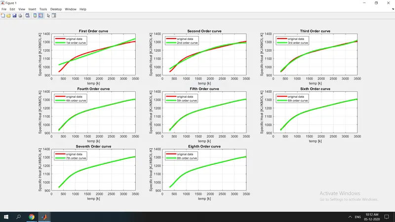
RMSE result :
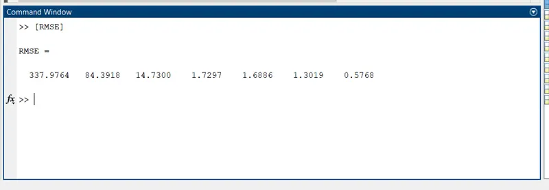
Conclusion: The curve to be goodfit the RMSE should tend to zero . From above RMSE output we can see that as we Increase the order of polynomial the value of RMSE tends to zero.
1.How to make a curve fit perfectly?
A curve can be made fit perfectly by Interpolation technique in which curve is drawn by intepolating point to point
2.How to get best fit?
A best fit can be obtained by increasing the order of polynomial .
3.What could be done to improve cubic fit?
A Cubic fit can be improved by choosing two different ordered polynomial i.e by splitting the curve.
References:
1.skill lync video lecture.
2. https://skill-lync.com/projects/Curve-Fitting-and-criterion-to-choose-best-fit-41860
3.https://skill-lync.freshdesk.com/support/solutions/articles/43000584172
4.https://skill-lync.com/knowledgebase/the-basic-concept-of-curve-fit