Week 4 - Genetic Algorithm

AIM- Write a code in MATLAB to optimise the stalagmite function and find the global maxima of the function

OBJECTIVE- 1. Explain the syntax for ga in MATLAB

2. Plot graphs for all 3 studies and for F maximum vs no. of iterations.

THEORY - A genetic algorithm is a search heuristic that is inspired by Charles Darwin’s theory of natural evolution. This algorithm reflects the process of natural selection where the fittest individuals are selected for reproduction in order to produce offspring of the next generation.

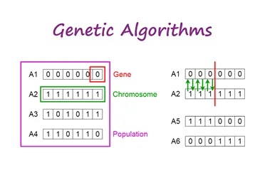
The process of natural selection starts with the selection of fittest individuals from a population. They produce offspring which inherit the characteristics of the parents and will be added to the next generation. If parents have better fitness, their offspring will be better than parents and have a better chance at surviving. This process keeps on iterating and at the end, a generation with the fittest individuals will be found.

This notion can be applied for a search problem. We consider a set of solutions for a problem and select the set of best ones out of them.

Five phases are considered in a genetic algorithm.

1. Initial population
2. Fitness function
3. Selection
4. Crossover
5. Mutation

1.Initial Population

The process begins with a set of individuals which is called a Population. Each individual is a solution to the problem you want to solve. An individual is characterized by a set of parameters (variables) known as Genes. Genes are joined into a string to form a Chromosome (solution). In a genetic algorithm, the set of genes of an individual is represented using a string, in terms of an alphabet. Usually, binary values are used (string of 1s and 0s). We say that we encode the genes in a chromosome.

2. Fitness Function

The fitness function determines how fit an individual is (the ability of an individual to compete with other individuals). It gives a fitness score to each individual. The probability that an individual will be selected for reproduction is based on its fitness score.

3. Selection

The idea of selection phase is to select the fittest individuals and let them pass their genes to the next generation. Two pairs of individuals (parents) are selected based on their fitness scores. Individuals with high fitness have more chance to be selected for reproduction.

Crossover is the most significant phase in a genetic algorithm. For each pair of parents to be mated, a crossover point is chosen at random from within the genes.

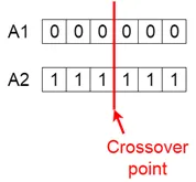
Offspring are created by exchanging the genes of parents among themselves until the crossover point is reached.

5. Mutation

In certain new offspring formed, some of their genes can be subjected to a mutation with a low random probability. This implies that some of the bits in the bit string can be flipped.

MAIN PROGRAM

clear all
close all
clc
% defining the values of x and y
x= linspace(0,0.6,200);
y=linspace(0,0.6,200);
% used to create a 2D mesh
[xx yy]= meshgrid(x,y)
%defining how many number of times ga should run
num_cases= 150;
f=get_stalagmite(x,y);
F = -f; % for obtaning the maximum
tic
%looping each cases and extrating the input and output for corresponding
%cases
%Study of statastical behaviour of GA in unbounded case
for i= 1: num_cases
    [inputs, fopt(i)]=ga(@peaks,2);
    xopt(i)=inputs(1);
    yopt(i)=inputs(2);
end
fopt = -fopt; %for plotting the maxima 
    study1_time=toc
   figure(1) 
   subplot(2,1,1)
   hold on
   surfc(x,y,F)
   shading interp
   plot3(xopt,yopt,fopt,'marker','o','markersize',5,'markerfacecolor','r')
   title('unbounded inputs')
   subplot(2,1,2)
   plot(fopt)
   xlabel('iterations')
   ylabel(' Function Maximum')
   
   %Study of statastical behaviour of GA when upper and lower bounds are
   %given
 
  tic
  for i= 1:num_cases
      [inputs,fopt(i)]= ga(@peaks,2,[],[],[],[],[0;0],[0.6;0.6]);
      xopt(i)=inputs(1);
      yopt(i)=inputs(2);
  end
     f=get_stalagmite(x,y);
   F= -f;
   
 
fopt = -fopt; %for plotting the maxima 
    study2_time=toc
   figure(2) 
   subplot(2,1,1)
   hold on
   surfc(x,y,F)
   shading interp
   plot3(xopt,yopt,fopt,'marker','o','markersize',5,'markerfacecolor','r')
   title('bounded inputs')
   subplot(2,1,2)
   plot(fopt)
   xlabel('iterations')
   ylabel(' Function Minimum')
   study_time2= toc
    
   options = optimoptions('ga','populationsize',250);
   f = get_stalagmite(x,y);
   F = -f
   tic
   for i = 1: num_cases
       [inputs,fopt(i)]= ga(@peaks,2,[],[],[],[],[0;0],[0.6;0.6],[],[],options);
       xopt(i) = inputs(1); 
       yopt(i) = inputs(2);
   end
   fopt = -fopt ;
   study_3_time = toc
   figure(3)
   subplot(2,1,1)
   hold on
   surfc(x,y,F)
   shading interp
   plot3(xopt,yopt,fopt,'marker','O','markersize',5,'markerfacecolor','r')
   title(' BOUNDED INPUTS WITH INCREASED POPULATION SIZE ')
   subplot(2,1,2)
   plot(fopt)
   xlabel('ITERATIONS')
   ylabel(' FUNCTION MAXIMUM ')

INPUTS FOR STALAGMITE FUNCTION

function [f]= get_stalagmite(x,y)
[xx,yy]= meshgrid(x,y);
 
for i= 1:length(xx);
   for j= 1: length(yy);
    input_vector(1)= xx(i,j);
    input_vector(2)=yy(i,j);
    f(i,j)= peaks(input_vector);
end
end
end

STALAGMITE FUNCTION FORMULATION

function [F]= peaks(input_vector)
x= input_vector(1);
y= input_vector(2);
 
f_1_x = (sin((5.1*pi*x)+0.5)).^6 ;
f_1_y = (sin((5.1*pi*y)+0.5)).^6 ;
f_2_x = exp((-4*log(2))*(x-0.00667).^2/0.64);
f_2_y = exp((-4*log(2))*(y-0.00667).^2/0.64);
 
F = -( f_1_x*f_1_y*f_2_x*f_2_y );
 
end

EXPLANATION OF CODE

1. First use the close all , clear all and clc command to clear the work space and command window.
2. Define the variable x & y using the linspace command (ie , we are creating an array for x and y each having 200 equally space values from 0 to 0.6 )
3. Now defining the number of cases or in other words we are defining the number of iterations for the program to run (ie how many times the program need to run before computing the results .
4. Now assigning the get_stalagmite function where inputs to the function is defined
5. Now assigning the " f " ( small f ) to the the variable " F" ( capital f) and calling the function ( ie stalagmite function) , and assigning F= - f ( cause thje objective of the program is to find the global maxima and ga command line only finds out minima and we know that the negative of minima is the global maxima of the function or model ) .
6. Now using the for loop and ga command line we are assigning for cases 1to 150 to the variable "i" the i value changes respectively.
7. As explained in the syntax for the ga command line we are giving the stalagmite function handle and no of variables as the input for the command line and the output of the command line is inputs and f val ( here the optimized results are assigned to the variable "fopt" ) , the command line is as follows " [inputs,fopt(i)] = ga(@stalagmite,2) " .
8. The fopt value changes with the variable i as for i = 1 to length(cases).
9. since we are finding out the maxima value we are plotting " - fopt " . using the plot command , shading interp command is used to smoothen the stalagmite plot. we are using the plot3 command to plot for xopt, yopt and fopt to plot the 3 plot .
10. For plotting all the variables we are using the hold on command . we are using the subplot command to plot the variance and optimization clearly as shown in the outputs.
11. tic and toc commands are used to compute the working time of the program.

CASE 2- In case 2 we are assigning the workspace for the optimisation function . In this case we are applying the bounds for the maxima ie we are saying the program to compute the maxima within the bounds given as input . The proccedure for case 2 is same follow all the steps till step 6 , only the ga command line is moddified as follows " [inputs,fopt(i)]= ga(@stalagmite,2,[],[],[],[],[0;0],[0.6;0.6]) " . Here [0;0] & [0.6;0.6] are given as upper and lower bounds respectively. Rest all other steps are same for the study of statistical behiviour of the stalagmite function.

CASE 3- In case 3 we are assigning the population size to the genetic algorithm command line , the syntax for it is as follows :1. " options = optimoptions('ga','populationsize',250) " . 2. Now assingn this options to the ga command line as shown " [inputs,fopt(i)]= ga(@stalagmite,2,[],[],[],[],[0;0],[0.6;0.6],[],[],options) " . by doing this we can compute and plot the exact maxima of the stalagmite function .

ERRORS OCCURRED AND RECTIFICATION

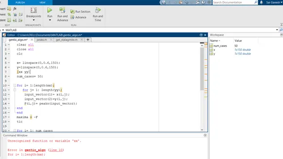
Meshgrid command is used to create a 2D array

2. Logical Error in finding the maxima

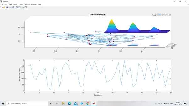
This is rectified by placing the minus sign.

3. Error with assignment operator

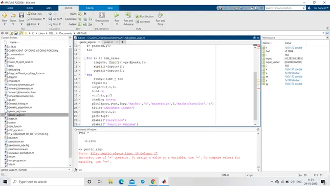
The symbol ‘-‘ is replaced with _ and the error is rectified.

RESULTS:

1. OPERATION OF GENETIC ALGORITHM WITHOUT ANY BOUNDARIES

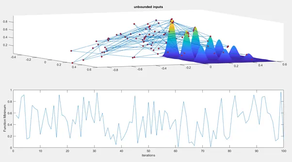
We can see that the ga command line plots the maxima all over the work space , the ga comand line computes the maxima but it has no bounds so it is very difficult to find the maxima from the above plot.

2. With Bounded Inputs

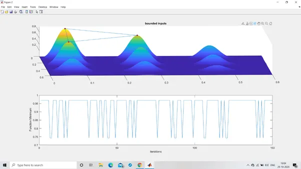
In case 2 we are specifying the bounds ie upper and lower bound in simple words we can say the we are specifying a workspace for the program to compute the output as result we can see that in figure 8 we get a cleaner plot showing the Maxima of the stalagmite function.

3. Including the population size

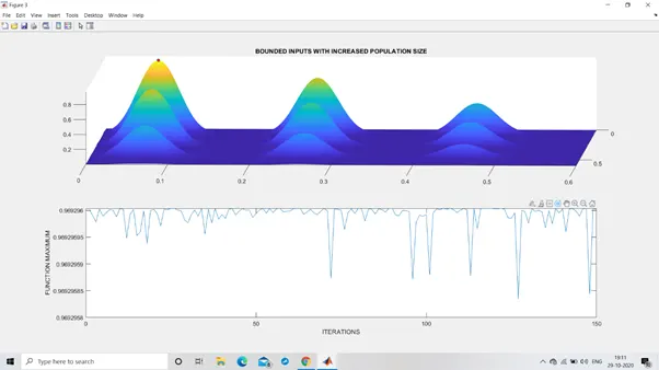
In order to get a exact plot for the global maxima we can increase the population size with the bounded constraints. The exact point of Maxima is computed.

From the above results we can conclude that: To get a narrower output we should

1. Increase the iterations
2. Increase the population size.
3. include the upper and lower bounds.

SYNTAX FOR GA

x = ga(fun,nvars,A,b,Aeq,beq,lb,ub,nonlcon,options) minimizes with the default optimization parameters replaced by values in options. (Set nonlcon=[] if no nonlinear constraints exist.)

options = optimoptions(SolverName,Name,Value) returns options with the named parameters altered with the specified values.

STOPPING CRITERIA FOR GA

The genetic algorithm uses the following options to determine when to stop. See the default values for each option by running opts = optimoptions('ga').

• MaxGenerations— The algorithm stops when the number of generations reaches MaxGenerations.
• MaxTime— The algorithm stops after running for an amount of time in seconds equal to MaxTime.
• FitnessLimit— The algorithm stops when the value of the fitness function for the best point in the current population is less than or equal to FitnessLimit.
• MaxStallGenerations— The algorithm stops when the average relative change in the fitness function value over MaxStallGenerations is less than Function tolerance.
• MaxStallTime— The algorithm stops if there is no improvement in the objective function during an interval of time in seconds equal to MaxStallTime.
• FunctionTolerance— The algorithm runs until the average relative change in the fitness function value over MaxStallGenerations is less than Function tolerance.
• ConstraintTolerance— The ConstraintTolerance is not used as stopping criterion. It is used to determine the feasibility with respect to nonlinear constraints. Also, max(sqrt(eps),ConstraintTolerance) determines feasibility with respect to linear constraints.

The algorithm stops as soon as any one of these conditions is met.

CONCLUSION

Thus the different variations of the outputs are observed with variations in different included parameters.