Week 3 - Solving second order ODEs

AIM: To write a Matlab program that solves the Differential Equations.

OBJECTIVE: 1. To solve the differential equation using Matlab

2. To create an animation that shows the variation of the position of the pendulum with respect to time

THEORY: A pendulum is a body suspended from a fixed support so that it swings freely back and forth under the influence of gravity. When a pendulum is displaced sideways from its resting, equilibrium position, it is subject to a restoring force due to gravity that will accelerate it back toward the equilibrium position. When released, the restoring force acting on the pendulum's mass causes it to oscillate about the equilibrium position, swinging it back and forth. The mathematics of pendulums is in general quite complicated. Simplifying assumptions can be made, which in the case of a simple pendulum allow the equations of motion to be solved analytically for small-angle oscillations.

A simple gravity pendulum is an idealized mathematical model of a real pendulum. This is a weight (or bob) on the end of a massless cord suspended from a pivot, without friction. Since in this model there is no frictional energy loss, when given an initial displacement it will swing back and forth at a constant amplitude. The model is based on these assumptions

• The rod or cord on which the bob swings is massless, inextensible, and always remains taut;
• The bob is a point mass;
• Motion occurs only in two dimensions, i.e. the bob does not trace an ellipse but an arc.
• The motion does not lose energy to friction.
• The gravitational field is uniform.
• The support does not move.

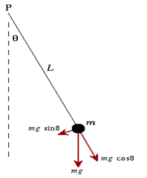
The below equation describes the ordinary differential equation that is obtained by solving the below free body diagram of the simple pendulum

`(d^2 θ)/(dt^2 )+(b/m) dθ/dt+(g(sinθ))/l=0`

Here In the above equation,

g = gravity in m/s2,

L = length of the pendulum in m,

m = mass of the ball in kg,

b=damping coefficient.

MAIN PROGRAM

clear all
close all
clc
b= 0.05; % damping coefficient
g=9.81;  % gravity in gravity in m/s2
l=1;    % length of the pendulum in m
m=0.1; %mass of the ball in kg
 
 
%initial condition
theta_0= [0;3]; % defining the initial values of position and velocity
%time points
t_span= linspace(0,20,500); % defining the integral values of limits
%solve ode
[t, results]= ode45(@(t,theta) ode_func(t,theta, b,g,l,m),t_span, theta_0) %definig the ode function
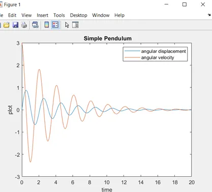
plot(t,results(:,1)) %plotting the time vs postion graph
hold on
plot(t,results(:,2)) %plotting the time vs velocity graph
hold on 
ylabel('plot') 
xlabel('time')
title(' Simple Pendulum')
legend('angular displacement','angular velocity')
 
    ct=1; % defining the counter and setting the inital value of the counter
   for i= 1:length(results(:,1)) %defining a or loop that iterates all the values of i upto the length of the results
        x=0; % defining the initial x coordinate value of the string
        y=0; % defining the initial y coordinate value of the string
        % defining the final x ad y coordinate values of the string
        x1=l*sin(results(i,1)) 
        y1=-l*cos(results(i,1))
        figure(2) %opens a new figure window
        plot([-2 2],[0 0],'linewidth',5) % plotting the fixed axis
        hold on
        plot([x x1],[y y1],'linewidth',3) % plotting the end line
        hold on
        plot([x1],[y1],'o','markersize',25,'markerfacecolor','b') %plotting the ball
        axis([-1 1 -1 1])
         pause(0.03) % defining the frequency at which the code is to be paused
        hold off
        M(ct)=getframe(gcf) % getting the individual frames and saving them in an array
        ct=ct+1; % for incrementing the counter 
      
       end
       
    % to create an animation
    movie(M)% to create a movie from the individual frames
    video= VideoWriter('pendulum.avi','Uncompressed AVI') %creates a video file from the array and control its properties
    open(video) % opens the video file
    writeVideo(video,M) % writing the movie in the videofile.
    close(video)% closes the video file

FUNCTION CODE

function [dtheta_dt]= ode_func(t,theta,b,g,l,m) %Defining the function that is called in the main program
 
theta1=theta(1)
theta2=theta(2)
%defining the values of theta 1 and theta 2
dtheta1_dt= theta2
dtheta2_dt= -(b/m)*theta2- (g/l)*sin(theta1)
dtheta_dt=[dtheta1_dt; dtheta2_dt]; % output definition in form of the column vector
end

EXPLANATION OF THE CODE

STEP 1: Define the values of the damping coefficient, the mass of the bob, gravity, and length of the string.

STEP 2: Define the initial conditions for Angular displacement and Angular velocity.

STEP 3: Using the linspace command create a time array that integrates the function

STEP 4: Create an ode function that solves the ordinary differential equation. Since the equation of the simple pendulum is a second-order ordinary differential equation we should break it into the two first-order differential equations. ode45(@(t,theta) ode_func(t,theta, b,g,l,m),t_span, theta_0).Here theta_0 is the initial values of the ode, t_span is the time to which the function is to be integrated. Ode_func is the user-defined function that contains all the necessary equations that are used to solve the ode. @ (t, theta) is the anonymous function and it gives the information to the program that these variables are not defined but acts as inputs. Here t is called the time step.

STEP 5: Plotting the results and labeling them using the commands plot and label

STEP 6: defining a for loop that iterates all the values of i up to the length of the results

By using the resolution of the vector, X0=0 is the initial x coordinate

Y0=0 is the initial y coordinate

x1=l*sin(results(i,1)) is the final X co-ordinate

Y1=-l*cos(results(i,1)) is the final y co-ordinate

Now plot the fixed axis and plot the line by using the above equations.

STEP 5: Introduce a pause and increment the value of the counter and for creating the movie get individual frames and save them in an array.

STEP 6: Create a video file and write the video.

ERRORS FACED AND RECTIFICATION OF ERRORS

1. This is a logical error I faced it corresponds to the resolution of the vector. The y coordinate of the line is entered as l*cos(results(i,1)) due to the pendulum rotated upwards

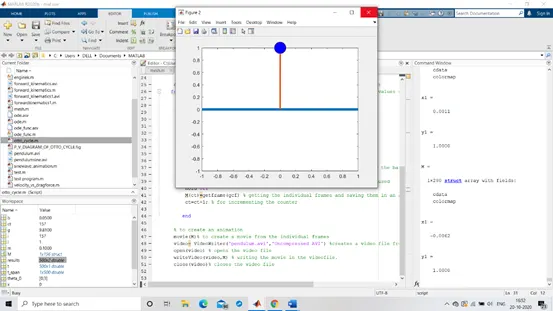
To rectify this a minus sign is introduced before and the equations turn out to be

-l*cos(results(i,1)).

2. A square matrix is introduced to have the marker but this shows a point in the space.

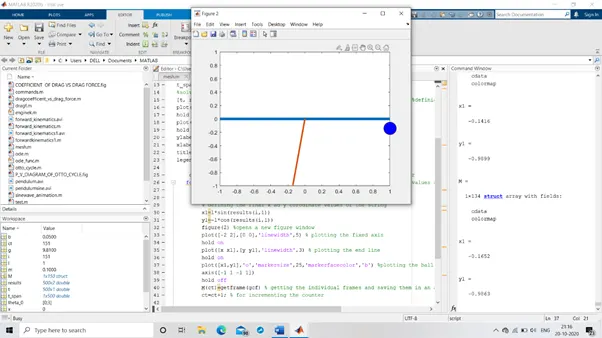
Removed the square braces and got the actual output.

RESULTS

The position of the pendulum with respect to the time is depicted in the link below.

https://youtu.be/wBADHClkE04

CONCLUSION

Thus the ordinary differential equation is solved by using the ode45 function and animation is made.