Week 4 - Genetic Algorithm
AIM - To optimize the stalagmite function and find the global maxima of the function.
OBJECTIVE- 1. Explain the concept of genetic algorithm and also the syntax for ga.
2. Plot graphs for all 3 studies and for F maximum vs no. of iterations.
INTRODUCTION -
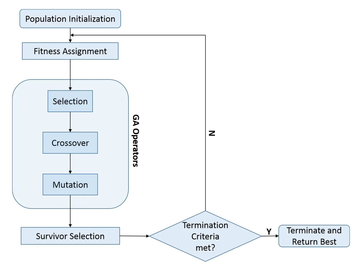
A genetic algorithm is a search heuristic that is inspired by Charles Darwin’s theory of natural evolution. This algorithm reflects the process of natural selection where the fittest individuals are selected for reproduction in order to produce offspring of the next generation.
The process of natural selection starts with the selection of fittest individuals from a population. They produce offspring which inherit the characteristics of the parents and will be added to the next generation. If parents have better fitness, their offspring will be better than parents and have a better chance at surviving. This process keeps on iterating and at the end, a generation with the fittest individuals will be found.
This notion can be applied for a search problem. We consider a set of solutions for a problem and select the set of best ones out of them.
Five phases are considered in a genetic algorithm.
- Initial population
- Fitness function
- Selection
- Crossover
- Mutation
INITIAL POPULATION
The process begins with a set of individuals which is called a Population. Each individual is a solution to the problem you want to solve.An individual is characterized by a set of parameters known as Genes. Genes are joined into a string to form a Chromosome.In a genetic algorithm, the set of genes of an individual is represented using a string, in terms of an alphabet. Usually, binary values are used. We say that we encode the genes in a chromosome.
FITNESS FUNCTION
The fitness function determines how fit an individual is (the ability of an individual to compete with other individuals). It gives a fitness score to each individual. The probability that an individual will be selected for reproduction is based on its fitness score.
SELECTION
The idea of selection phase is to select the fittest individuals and let them pass their genes to the next generation.Two pairs of individuals (parents) are selected based on their fitness scores. Individuals with high fitness have more chance to be selected for reproduction.
CROSSOVER
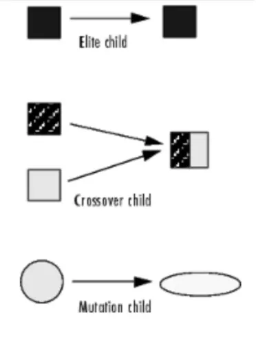
Crossover is the most significant phase in a genetic algorithm. For each pair of parents to be mated, a crossover point is chosen at random from within the genes.
MUTATION
In certain new offspring formed, some of their genes can be subjected to a mutation with a low random probability. This implies that some of the bits in the bit string can be flipped.Mutation occurs to maintain diversity within the population and prevent premature convergence. The algorithm terminates if the population has converged (does not produce offspring which are significantly different from the previous generation). Then it is said that the genetic algorithm has provided a set of solutions to our problem.
FLOW DIAGRAM-
SYNTAX FOR GA
Syntax

x = ga(fun,nvars)
x = ga(fun,nvars,A,b)
x = ga(fun,nvars,A,b,Aeq,beq)
x = ga(fun,nvars,A,b,Aeq,beq,lb,ub)
x = ga(fun,nvars,A,b,Aeq,beq,lb,ub,nonlcon)
x = ga(fun,nvars,A,b,Aeq,beq,lb,ub,nonlcon,options)
x = ga(fun,nvars,A,b,[],[],lb,ub,nonlcon,IntCon)
x = ga(fun,nvars,A,b,[],[],lb,ub,nonlcon,IntCon,options)
x = ga(problem)
[x,fval] = ga(___)
[x,fval,exitflag,output] = ga(___)
[x,fval,exitflag,output,population,scores] = ga(___)
INPUT FUNCTION
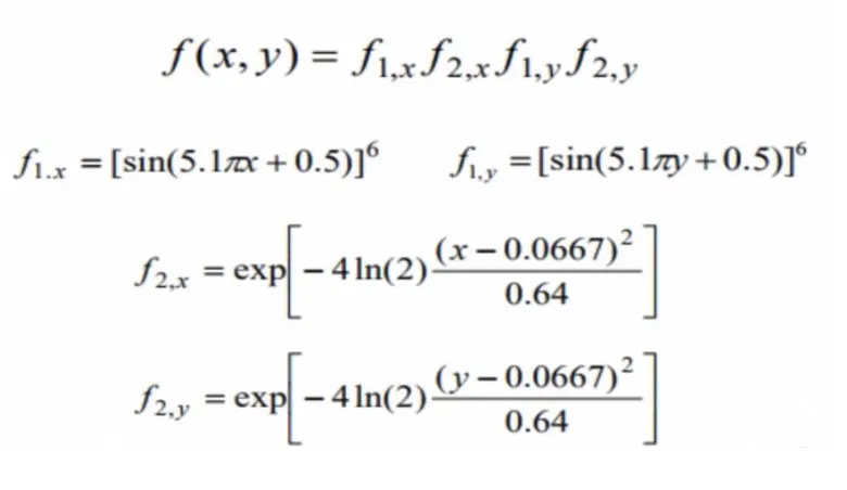
The above equation is used in the stalagmite functions and is used to plot the graph
function [f]= stalagmite(input_vector)

% x and y is the input parameter
x=input_vector(1);
y=input_vector(2);

f1=(sin(5.1*pi*x+0.5)).^6;
f2=exp(-4.*log(2)*((x-0.0667).^2./0.64));
f3=(sin(5.1*pi.*y+0.50)).^6;
f4=exp(-4*log(2)*((y-0.0667).^2./0.64));


f=-(f1.*f2.*f3.*f4);   % Negative sign is used to reverse the plot for finding maxima

end
MAIN BODY
clear all
close all
clc

%defining our search space
x= linspace(0,0.6,150);
y= linspace(0,0.6,150);

%creating a 2Dimensional mesh
[xx yy]= meshgrid(x,y);

%no of iterations for which the function will evaluate the function
num_cases=50;

%evaluating the stalagmite function
for i = 1:length(xx)
  for j = 1:length(yy)
     input_vector(1)=xx(i,j);
     input_vector(2)=yy(i,j);
     f(i,j) = stalagmite(input_vector);  %values of function in given search space
  end

end


surf(xx,yy,-f);   %generating the surface
shading interp    %to remove the lines produced by the mesh grid
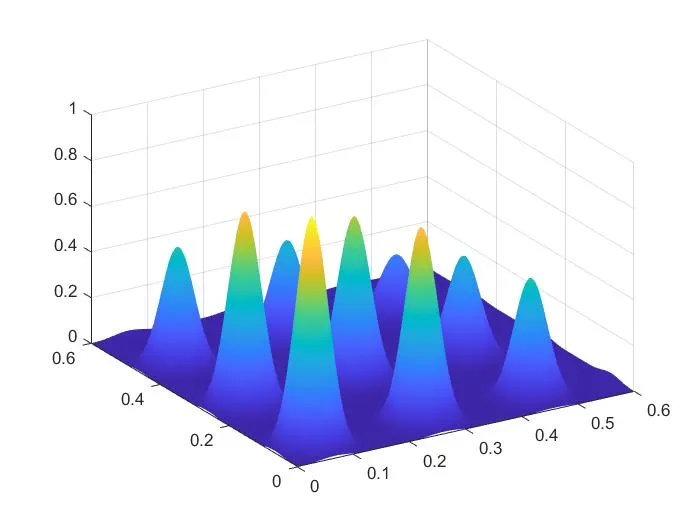
The plot generated is shown below
MAIN CODE
clear all
close all
clc

%defining our search space
x= linspace(0,0.6,150);
y= linspace(0,0.6,150);

%creating a 2Dimensional mesh
[xx, yy]= meshgrid(x,y);

%no of iterations for which the function will evaluate the function
num_cases=50;

%evaluating the stalagmite function
for i = 1:length(xx)
  for j = 1:length(yy)
     input_vector(1)=xx(i,j);
     input_vector(2)=yy(i,j);
     f(i,j) = stalagmite(input_vector);  %values of function in given search space
  end

end


surf(xx,yy,-f);   %generating the surface
shading interp    %to remove the lines produced by the mesh grid


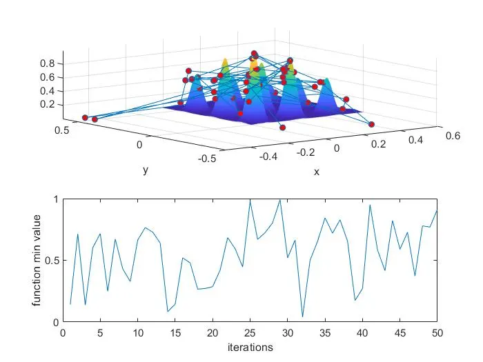
%Unbounded Statistical behaviour

tic                   %caluculating the study time by using tic n toc command
for i=1:num_cases
    [inputs,fopt1(i)] = ga(@stalagmite,2);  %calculating the optimized value of the function
    xopt(i)=inputs(1);
    yopt(i)=inputs(2);
end
study_time1=toc;

figure(1)

subplot(2,1,1)

surfc(x,y,-f);
hold on
shading interp
plot3(xopt,yopt,-fopt1,'Marker','o','MarkerSize',5,'MarkerFaceColor','r');
xlabel('x');
ylabel('y');
grid on
subplot(2,1,2);
plot(-fopt1);
xlabel('iterations')
ylabel('function min value')


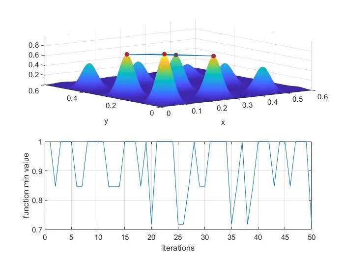
%Bounded Statistical behaviour
tic                      %calculating the study time by using tic n toc command
for j=1:num_cases
 [inputs,fopt2(j)] = ga(@stalagmite,2,[],[],[],[],[0;0],[1;1]);%calculating the
                                                   %optimized value of the function
  xopt(j)=inputs(1);
  yopt(j)=inputs(2);
end
study_time2=toc;

figure(2)

subplot(2,1,1)

surfc(x,y,-f);
hold on
shading interp
plot3(xopt,yopt,-fopt2,'Marker','o','MarkerSize',5,'MarkerFaceColor','r');
xlabel('x');
ylabel('y');
grid on
subplot(2,1,2);
plot(-fopt2);
xlabel('iterations')
ylabel('function min value')
grid on


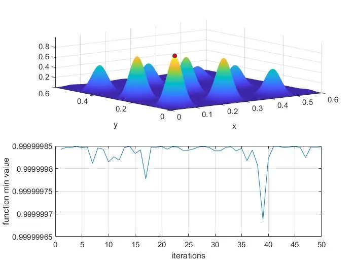
%Statistical data using the Increased Population Size

options=optimoptions('ga');    %increasing the population size by using optimoptions command
options=optimoptions(options,'PopulationSize',300);

tic           %caluculating the study time by using tic n toc command
for j=1:num_cases
    [inputs,fopt3(j)] = ga(@stalagmite,2,[],[],[],[],[0;0],[1;1],[],[],options);
    xopt(j)=inputs(1);
    yopt(j)=inputs(2);
end
study_time3=toc;

figure(3)

subplot(2,1,1)

surfc(x,y,-f);
hold on
shading interp
plot3(xopt,yopt,-fopt3,'Marker','o','MarkerSize',5,'MarkerFaceColor','r');
xlabel('x');
ylabel('y');
grid on
subplot(2,1,2);
plot(-fopt3);
xlabel('iterations')
ylabel('function min value')
grid on

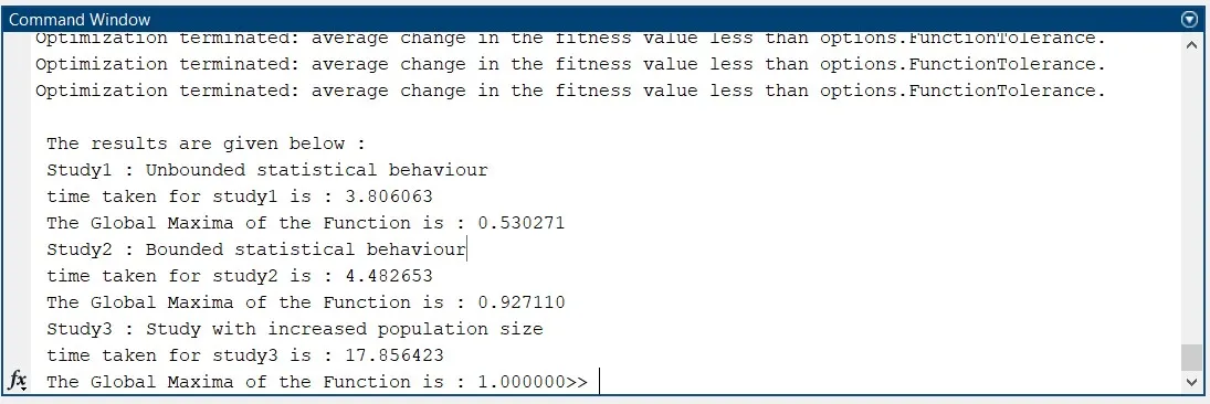
fprintf('\n Study1 : Unbounded statistical behaviour')
fprintf('\n time taken for study1 is : %f',study_time1)
fprintf('\n The Global Maxima of the Function is : %f',-(mean(fopt1)))

fprintf('\n Study2 : Bounded statistical behaviour')
fprintf('\n time taken for study2 is : %f',study_time2)
fprintf('\n The Global Maxima of the Function is : %f',-(mean(fopt2)))

fprintf('\n Study3 : Study with increased population size')
fprintf('\n time taken for study3 is : %f',study_time3)
fprintf('\n The Global Maxima of the Function is : %f',-(mean(fopt3)))
PLOT FOR UNBOUNDED STATISTICAL BEHAVIOUR
PLOT FOR BOUNDED STATISTICAL BEHAVIOUR
PLOT FOR STUDY WITH INCREASING POPULATION SIZE
STALAGMITE FUNCTION OUTPUT -
REFERENCES-
https://in.mathworks.com/help/gads/ga.html#responsive_offcanvas