Week 3 - Solving second order ODEs

AIM - To solve the Second Order ODE Function using the MATLAB which depicts the motion of Pendulum.

OBJECTIVE - To write a program for the ODE that represents the motion of the pendulum with simple damping

THEORY-

A pendulum is a weight suspended from a pivot so that it can swing freely. When a pendulum is displaced sideways from its resting, equilibrium position, it is subject to a restoring force due to gravity that will accelerate it back toward the equilibrium position. When released, the restoring force acting on the pendulum's mass causes it to oscillate about the equilibrium position, swinging back and forth. The time for one complete cycle, a left swing and a right swing, is called the period. The period depends on the length of the pendulum and also to a slight degree on the amplitude, the width of the pendulum's swing.

The ODE equation is as follows

`(d^2theta)/dt^2+b/m*((d.theta)/dt)+g/L(sintheta)=0`

where g= gravity in m/s^2

m= mass of the ball 1 kg

b =Damping coefficient

L= length of the pendulum in m

The Fixed Parameters given were

Length(L) = 1m

Mass of the ball(m) = 1kg

Gravity(g) = 9.81

Damping coefficient(b) = 0.05

Time period = 0-20 sec

Angular Velocity = 3rad/sec at time t=0

Angular Displacement = 0

MAIN PROGRAM

clear all
close all
clc


b=0.05;  %damping coefficient
g=9.81;  %Gravity in m/s^2
l=1;     %length in meters 
m=1;   %mass of pendulum in kg

%initial condition
theta_0 = [0;3];         %angular velocity=3,angular displacement=0

%time points
t_span = linspace(0,20,100);

%solve ODE
[t,results] = ode45(@(t,theta) ode_func(t,theta,b,g,l,m),t_span,theta_0);

plot(t,results(:,1))
hold on
plot(t,results(:,2))
xlabel('time')
ylabel('Velocity and Displacement')
legend('Displacment','velocity')
grid on


%animation


ct =1
for i=1:length(results(:,1))
    
    x0=0;
    y0=0;
    
    x1=l*sin(results(i,1)+pi);
    y1=l*cos(results(i,1)+pi);
    
    figure(2)
    
    plot([x0 x1],[y0 y1],'-o','MarkerSize',10,'linewidth',5)
    axis([-2 2 -2 2])
    hold on
    plot([-1 1],[0 0],'linewidth',3,'color','r')
    hold off
    pause(0.003)
    M(ct) = getframe(gcf);
    ct=ct+1;
    
end

movie(M)
videofile= VideoWriter('mains.avi','uncompressed AVI')
open(videofile)
writeVideo(videofile,M)
close(videofile)

FUNCTION CODE

function [a]= ode_func(t,theta,b,g,l,m)

theta1=theta(1)
theta2=theta(2)
dtheta1_dt = theta2;
dtheta2_dt = -(b/m)*theta2 - (g/l)*sin(theta1);
dtheta_dt = [dtheta1_dt; dtheta2_dt]

end

PROCEDURE-

1.In this project the fixed parameters such as the length,mass,damping coefficient and the acceleration due to gravity were given.

2.Also the time and the angles were given as the initial condition.

3.Using the tspan command,100 values were taken in between the 0 to 20 times period.

4.Using the ode45 command the ODE function was introduced.

5.Plot command was then used to plot the velocity and displacement vs time graph.

6.For loop command was then used to plot the mass at various points and time to plot the graph.

7.In the end using the movie command the videofile was created and then plot is saved as the uncompressed.avi file

PLOT

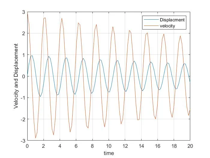
OUTPUT ANIMATION

The videofile created for the plot was uploaded and the link to the video is given below

https://youtu.be/JxZ1wsokR8o