Genetic Algorithm

Aim: Write a code in MATLAB to optimise the stalagmite function and find the global maxima of the function.

Objective:

1. Write the stalagmite function in MATLAB.

2. Program for optimizing stalagmite function using Genetic Algorithm.

3. Plot graphs of Maximum function vs no. of iterations for all 3 studies (unbounded inputs, bounded inputs and increased population).

Theory:

Genetic Algorithm is optimization method based on the mechanics of natural genetics and natural selection. Genetic Algorithm is used for scheduling to find the near to optimum solution in short time. In general, Genetic Algorithm is used as tool in different processes to optimize the process parameters. Genetic algorithms are inspired by Darwin theory about evolution Survival of The Fittest. The genetic algorithm repeatedly modes a population of individual solutions. At each step, the genetic algorithm selects individuals at random from the current population to be parents and uses them to produce the children for the next generation. Over successive generations, the population "evolves" toward an optimal solution. You can apply the genetic algorithm to solve a variety of optimization problems that are not well suited for standard optimization algorithms, including problems in which the objective function is discontinuous, nondifferentiable, stochastic, or highly nonlinear. The genetic algorithm can address problems of mixed integer programming, where some components are restricted to be integer-valued.

Every living organism consist of cells, that describe how that organisms built. Each cell has same set of Chromosomes. A Chromosomes consist of genes and DNA blocks, hereditary factors that determine particular traits of an individual are encoded into the genes and forming DNA blocks which are strung along the length of chromosomes. Each traits of an individual encoded by some combination of DNA. Complete set of genetic material is called genome particular set of genes in genome is called genotype. The physical expression of the genotype is called the phenotype, its physical and mental characteristics, such as eye colour, intelligence etc. This is called as reproduction. When two phenotypes (two organism) where mate they share their genes; the resultant offspring may end up having half the genes from one organism and half from other. This is called as crossover. Mutations mean change in element of DNA. This change is mainly caused by errors in copying genes from parents.

What is Stalagmite function?

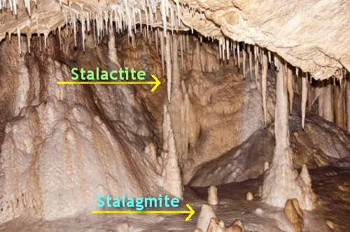
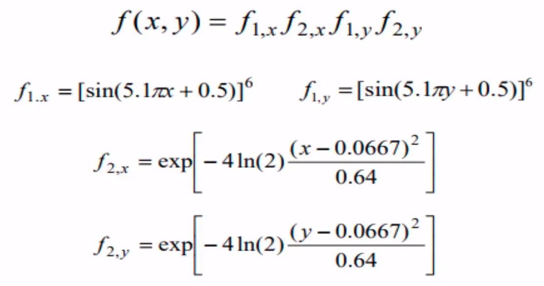
Stalagmite is a type of rock formation that rises from the floor of a cave due to the accumulation of material deposited on the floor from ceiling drippings. Stalagmites are typically composed of calcium carbonate, but may consist of lava, mud, peat, pitch, sand, sinter. A close identical geometrical shape can be obtained by using a mathematical function. This function should be applied to two variables in two dimensions which yields the stalagmite. It can be mathematically expressed as below.

STEP-1: Write the stalagmite function in MATLAB

%Stalagmite function
function [F] = stalagmite_ip(inputs)
x = inputs(1);
y = inputs(2);
fx1 = (sin((5.1*pi).*x+0.5)).^6;
fx2 = exp((((x-0.0667).^2)/0.64).*(-4*log(2)));
fy1 = (sin((5.1*pi).*y+0.5)).^6;
fy2 = exp((((y-0.0667).^2)/0.64).*(-4*log(2)));
F = -1*fx1*fx2*fy1*fy2;
end

STEP-2 & 3: Program for optimizing stalagmite function using Genetic Algorithm. Plot graphs of Maximum function vs no. of iterations for all 3 studies

Case-1. Unbounded Inputs

%Start Of the Program

close all
clear all
clc

x=linspace(0,0.6,150);
y=linspace(0,0.6,150);
num_cases=30;

%Creating 2D array using meshgrid function
[xx yy]=meshgrid(x,y);

%Nested loop for array value input

for i=1:length(xx)
    for j=1:length(yy)
        inputs(1)=xx(i,j);
        inputs(2)=yy(i,j);
       f(i,j)= stalagmite_ip(inputs);
    end
end

tic
for i=1:num_cases
[inputs,fopt1(i)]=ga(@stalagmite_ip,2);
xopt(i)=inputs(1);
yopt(i)=inputs(2);
end

case_1=toc
fopt1 = -1*fopt1;
f = -f;
figure(1)
subplot(2,1,1)
surfc(xx,yy,f)
xlabel('x value')
ylabel('y value')
title('Unbounded Inputs','color','k')
shading interp
hold on;
plot3(xopt,yopt,fopt1,'marker','o','markersize',5,'markerfacecolor','r');
subplot(2,1,2)
plot(fopt1);
xlabel('Iterations')
ylabel('Max Function') 

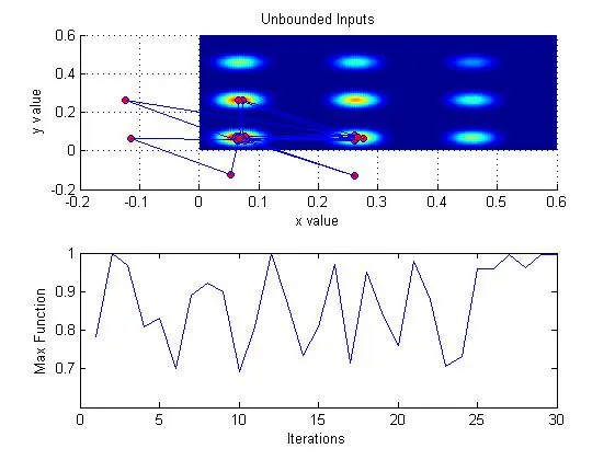
Result: Graph of Max. function vs No. of iterations

Case-2: Bounded Inputs

%Start Of the Program

close all
clear all
clc

x=linspace(0,0.6,150);
y=linspace(0,0.6,150);
num_cases=30;

%Creating 2D array using meshgrid function
[xx yy]=meshgrid(x,y);

%Nested loop for array value input

for i=1:length(xx)
    for j=1:length(yy)
        inputs(1)=xx(i,j);
        inputs(2)=yy(i,j);
       f(i,j)= stalagmite_ip(inputs);
    end
end

 tic
for i=1:num_cases
[inputs,fopt2(i)]=ga(@stalagmite_ip,2,[],[],[],[],[0;0],[0.5;0.5]);
xopt(i)=inputs(1);
yopt(i)=inputs(2);
end

fopt2 = -1*fopt2;
case_2=toc
figure(2)
subplot(2,1,1)
surfc(xx,yy,f)
xlabel('x value')
ylabel('y value')
title('Bounded Inputs','color','k')
shading interp
hold on;
plot3(xopt,yopt,fopt2,'marker','o','markersize',5,'markerfacecolor','r');
subplot(2,1,2)
plot(fopt2);
xlabel('Iterations')
ylabel('Max Function') 

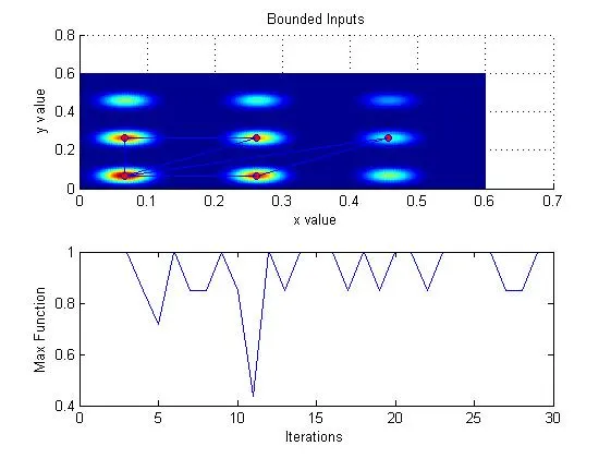
Result: Graph of Max. function vs No. of iterations

Case-3: Bounded with increased population size

%Start Of the Program

close all
clear all
clc

x=linspace(0,0.6,150);
y=linspace(0,0.6,150);
num_cases=30;

%Creating 2D array using meshgrid function
[xx yy]=meshgrid(x,y);

%Nested loop for array value input

for i=1:length(xx)
    for j=1:length(yy)
        inputs(1)=xx(i,j);
        inputs(2)=yy(i,j);
       f(i,j)= stalagmite_ip(inputs);
    end
end

options = gaoptimset('ga');
options = gaoptimset(options,'PopulationSize',170);
  
for i=1:num_cases
[inputs,fopt3(i)]= ga(@stalagmite_ip,2,[],[],[],[],[0;0],[0.5;0.5],[],[],options);
xopt(i)=inputs(1); 
yopt(i)=inputs(2);
end

fopt3 = -1*fopt3;
case_3=toc
figure(3)
subplot(2,1,1)
surfc(xx,yy,f)
xlabel('x value')
ylabel('y value')
title('Bounded Inputs with modified population size','color','k')
shading interp
hold on;
plot3(xopt,yopt,fopt3,'marker','o','markersize',5,'markerfacecolor','r');
subplot(2,1,2)
plot(fopt3);
xlabel('Iterations')
ylabel('Max Function') 

%Displaying the values of x & y for Max. function value
display(inputs)

Result: Graph of Max. function vs No. of iterations

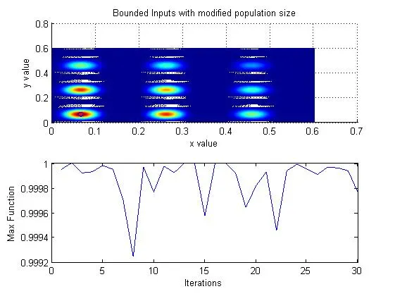
Conclusion:

Max. function values of x & y: