Solving second order ODEs

Aim: Simulation of simple pendulum using ODE and Matlab program

Given: Equation of motion of a simple pendulum with damping using Newton's II law is,

`(d^2theta)/(dt^2)+(c/m)(d theta)/dt+(g/l)sin(theta)=0`

from the above equation, transform into two ODE,

`(d theta1)/dt = theta2` and

`(d theta2)/dt = (-c/m(theta2) - g/lsin(theta1))`

In matrix form,

`[(d theta)/dt] = [(d theta1)/dt ; (d theta2)/dt]`

In the above equation, where

g = 9.81m/sec^2 = acceleration due to gravity in m/sec^2,

L = 1 meter = length of the pendulum in m,

m = 1 kg = mass of the ball in kg,

c = 0.05 = damping coefficient.

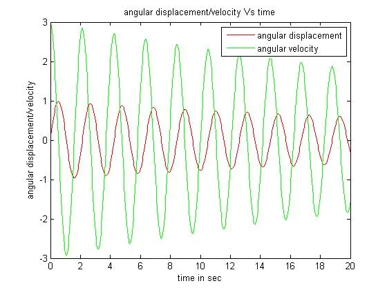
Simulate the motion between 0-20 sec, for angular displacement=0,angular velocity=3 rad/sec at time t=0.

Codes for calling function:

%ODE fuction created for simple pendulum
function [dtheta_dt] = ode_func(t, theta, c, g, l, m)
theta1 = theta(1)
theta2 = theta(2)
dtheta1_dt = theta2;
dtheta2_dt = -(c/m)*theta2 -(g/l)*sin(theta1);
dtheta_dt = [dtheta1_dt; dtheta2_dt];
end

Codes for simulation of simple pendulum:

%simulation of simple pendulum
close all
clear all
clc

%inputs of simple pendulum
c = 0.05; %damping coeffcicient
g = 9.81; %acceleration due to gravity
l = 1; %length of the pendulum
m = 1; %bob mass

%initial condition
theta_0 = [0;3]; %initial angular displacement & angular velocity

%time steps
t_span = linspace(0,20,500);

%solve ODE
[t,results] = ode45(@(t,theta) ode_func(t, theta, c, g, l, m), t_span, theta_0);

%plotting
figure(1)
plot(t,results(:,1),'color','r');
hold on
plot(t, results(:,2),'color','g');
%x & Y label & title name
xlabel('time in sec')
ylabel('angular displacement/velocity')
%legend name
legend('angular displacement','angular velocity')
%title of the graph
title('angular displacement/velocity Vs time')

%simultation of pendulum
%for statement
ct=1; %variable that simply increment or decrement by specific step in every iteration
for i = 1:length(results(:,1))
    %coordinate values
    %pivot point
    x0 = 0;
    y0 = 0;
    %pendulum length
    x1 = l*sin(results(i,1));
    y1 = -l*cos(results(i,1));
    
    %output
    %plotting of simple pendulum
    figure(2)
    %initial & final value of x & y with linewidth of 3
    plot([x0 x1], [y0 y1],'linewidth',3)
    hold on
    plot(x1, y1,'o','markers',15,'markerfacecolor','g') %bob at free end
    plot(x0, y0,'o','markers',5,'markerfacecolor','r') %at fixed end
    %simple pendulum movement value
    axis([-1.5 1.5 -1.2 0.2]);
    hold off
    pause(0.08); %control movie frames
    M(ct) = getframe(gcf); %get array of movie frame
    ct=ct+1; %inrement by every iteration or loop
end

%creating movie
movie(M)
videofile = VideoWriter('simple_pendulum.avi') %create video file
open(videofile) %open videofile once it generate
writeVideo(videofile, M) %create video file from an array or M file
close(videofile) %close video file

Result:

1. Graph of angular displacement/velocity Vs time with an angular displacement is zero and angular velocity is 3 rad/sec for t=0 sec.

2. Simulation of simple pendulum (Google drive link) : https://drive.google.com/file/d/1FBt-j1E-hY8bWi4ubNGidZtKL3gdXAhm/view?usp=sharing