Project 2 - Rankine cycle Simulator

Aim: Simulate the Rankine cycle using MATLAB.

Objective:

1. Calculate the state point of the Rankine cycle based on user input (XSteam library) using MATLAB.

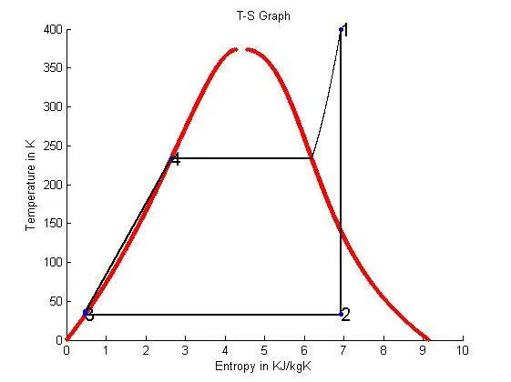
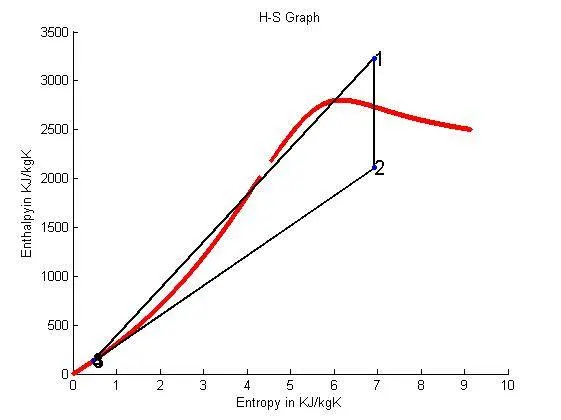
2. Plot the corresponding T-s and h-s plots for the given set of inputs.

Theory:

The Rankine cycle is a model used to predict the performance of steam turbine systems. It was also used to study the performance of reciprocating steam engines. The Rankine cycle operates in the following steps:

Process 1-2: Isentropic compression in a pump.

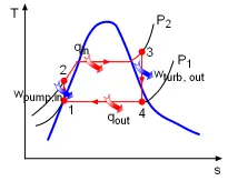
w_{pump, in} = h₂ - h₁

Process 2-3: Constant pressure heat addition in a boiler.

q_in = h₃ - h₂

Process 3-4: Isentropic expansion in a turbine.

w_{turbine, out} = h₃ - h₄

Process 4-1: Constant pressure heat rejection in a condenser.

q_out = h₄ - h₁

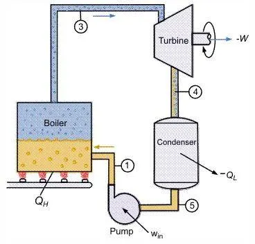
T-s and h-s Graph of Rankine cycle:

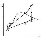
STEP-1: Calculation of four different state point of Rankine cycle using MATLAB

Given inputs:

Turbine Inlet temperature = 400° C

Turbine Inlet Pressure = 30 bars

Turbine Outlet Pressure (Condenser Inlet Pressure)= 0.05 bars

%Rankine cycle simulation
clear all
close all
clc

%Heading
disp('           RANKINE CYCLE SIMULATION        ');

%Process of Rankine cycle
disp('1-2 is Isentropic Expansion in the Turbine');
disp('2-3 is Constant Pressure Heat Rejection by the Condensor');
disp('3-4 is Isentropic Compression in the Pump');
disp('4-1 is Constant Pressure Heat Addition by the Boiler'); 
fprintf('\n');

%Input values of temperature and pressure
P1 = input('Enter the Turbine inlet Pressure (in bar):    '); %Inlet pressure at state 1
T1 = input('Enter the Turbine inlet Temperature(in Degree Celsius):  '); %Inlet temperature at state 1  
P2 = input('Enter the Turbine outlet(Condenser inlet pressure)(in Bar):  '); %outlet pressure at state 2  
fprintf('\n');

%Properties Calculation 
%Calculation of Enthalpy at saturation points 1,2,3 & 4
H1 = XSteam('hV_p',P1);
H2 = XSteam('hV_p',P2);
H3 = XSteam('hL_p',P1);
H4 = XSteam('hL_p',P2);

%Calculation of Entropy at saturation points 1,2,3 & 4
S1 = XSteam('sV_p',P1);
S2 = XSteam('sV_p',P2);
S3 = XSteam('sL_p',P1);
S4 = XSteam('sL_p',P2);

%calculation of saturation temperature at Pressure
T_sat1 = XSteam('Tsat_p',P1);
T_sat2 = XSteam('Tsat_p',P2);

%Process of four dissferent states
fprintf('Results\n')
%State-1
fprintf('At state point-1\n');
h1 = XSteam('h_pT',P1,T1);
s1 = XSteam('s_pT',P1,T1);
fprintf('P1 is :%0.2f bar\n',P1);
fprintf('T1 is :%0.2f degC\n',T1);
fprintf('H1 is :%0.2f KJ/Kg\n',h1);
fprintf('S1 is :%0.2f KJ/KgK\n\n',s1);

%State-2
fprintf('At satate point-2\n');
s2 = s1;
X = (s2-S4)/(S2-S4); % Dryness fraction 
h2 = H4 + X*(H2-H4);  
T2 = XSteam('T_ph',P2,H2); 
fprintf('P2 is :%0.2f bar\n',P2);
fprintf('T2 is :%0.2f degC\n',T2);
fprintf('H2 is :%0.2f KJ/Kg\n',h2);
fprintf('S2 is :%0.2f KJ/KgK\n\n',s2);

%State-3
fprintf('At satate point-3\n');
P3 = P2;
T3 = T_sat2;
h3 = H4;
s3 = S4;
fprintf('P3 is :%0.2f bar\n',P3);
fprintf('T3 is :%0.2f degC\n',T3);
fprintf('H3 is :%0.2f KJ/Kg\n',h3);
fprintf('S3 is :%0.2f KJ/KgK\n\n',s3);

%State-4
fprintf('At satate point-4\n');
P4 =P1;
s4 = s3;
%Calculation of Specific heat value 
Cp_1 = XSteam('Cp_ps',P4, s4);
Cv_1 = XSteam('Cv_ps',P4, s4);
gama = Cp_1/Cv_1;
k = (gama-1)/gama;
T4 = T3*(P4/P3)^k;
h4 = XSteam('H_ps',P4,s4);
fprintf('P4 is :%0.2f bar\n',P4);
fprintf('T4 is :%0.2f degC\n',T4);
fprintf('H4 is :%0.2f KJ/Kg\n',h4);
fprintf('S4 is :%0.2f KJ/KgK\n\n',s4);

%Turbine & Pump work
w_turbine = h1 - h2;
w_pump    = h4 - h3;
%Net work
w_net = w_turbine - w_pump;
%Heat supplied
Q_supplied = h1 - h4;
%efficiency
eta = (w_net/Q_supplied)*100;
%Back work ratio
BW_Ratio = w_pump/w_turbine;
%Steam rate
s_rate = 3600/(w_turbine - w_pump);
fprintf('Wt is :%0.2f KJ/Kg\n',w_turbine);
fprintf('Wp is :%0.2f KJ/Kg\n',w_pump);
fprintf('Wnet is :%0.2f KJ/Kg\n',w_net);
fprintf('BWR is :%0.2f\n',BW_Ratio);
fprintf('Ntherm is :%0.2f percent\n',eta);
fprintf('S.S.C is :%0.2f Kg/KWh\n\n',s_rate);

%Plotting T-S and H-S graph
%plot of T-S graph
temp = linspace(0,T1,1000);
figure(1)
hold on  
for i = 1:length(temp)
    plot(XSteam('sL_T',temp(i)),temp(i),'r.')
    plot(XSteam('sV_T',temp(i)),temp(i),'r.')
end 
plot([s1 s2],[T1 T2],'linewidth',2,'color','k',...
    'marker','o','markersize',3,'markerfacecolor','b','markeredgecolor','b')
text(s1,T1,'1','FontSize',15);
text(s2,T2,'2','FontSize',15);
plot([s2 s3],[T2 T3],'linewidth',2,'color','k','marker','o','markersize',3,'markerfacecolor','b','markeredgecolor','b');
text(s3,T3,'3','FontSize',15);
plot([s4 S3],[T4 T_sat1],'linewidth',2,'color','k','marker','o','markersize',3,'markerfacecolor','b','markeredgecolor','b');
text(S3,T_sat1,'4','FontSize',15);
%process 4-1 vapour line
x = linspace(T_sat1,T1,1000); 
for i = 1:length(x)
    plot(XSteam('s_pT',P1,x(i)),x(i),'linewidth',6,'color','k')
end 
plot([S3 S1],[T_sat1 T_sat1],'linewidth',2,'color','k')
xlabel('Entropy in KJ/kgK') 
ylabel('Temperature in K')
title('T-S Graph') 

%plot of H-S graph
figure(2) 
hold on
for i = 1:length(temp)
     plot(XSteam('sL_T',temp(i)),XSteam('hL_T',temp(i)),'r.')
     plot(XSteam('sV_T',temp(i)),XSteam('hV_T',temp(i)),'r.')
end
plot([s1 s2 s3 s4 s1],[h1 h2 h3 h4 h1],'linewidth',2,'color','k',...
    'marker','o','markersize',3,'markerfacecolor','b','markeredgecolor','b')
text(s1,h1,'1','FontSize',15)
text(s2,h2,'2','FontSize',15)
text(s3,h3,'3','FontSize',15)
text(s4,h4,'4','FontSize',15)
xlabel('Entropy in KJ/kgK') 
ylabel('Enthalpyin KJ/kgK')
title('H-S Graph')

Result:

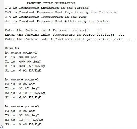
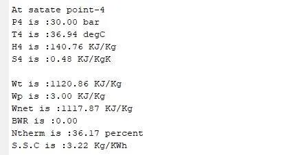
Graph of T-s and H-s with given user inputs:

Conclusion:

1. Simulation of Rankine cycle has done based on user inputs and XSteam library using MATLAB.

2. Finally, Graph of T-s and H-s is plotted for Rankine cycle.

References:

1. http://thermopedia.com

2. http://www.ecourses.ou.edu/cgi-bin/ebook.cgi?topic=th&chap_sec=10.1&page=theory.