Week 4 - Genetic Algorithm

Objective: To write a Matlab code to optimize the stalagmite function and to find the global maxima using the genetic algorithm comment.

Theory:

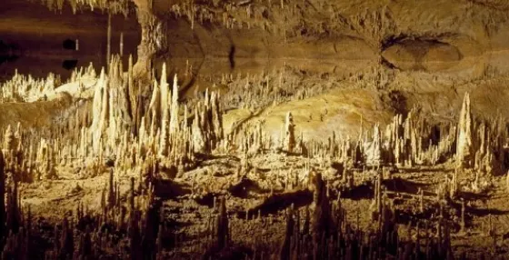
Stalagmite function: Stalagmite is a type of rock formation that rises from the floor of a cave due to the accumulation of mineral deposits as shown below.

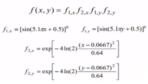
The stalagmite function (shown below) is a mathematical equation whose results also produce a similar kind of structure in the graph,

Optimization: This process helps to identify the best possible solutions (close to ideal condition) in an iterative method, within the given initial conditions and constraints. The below graph is an overview of how the Optimization process is done.

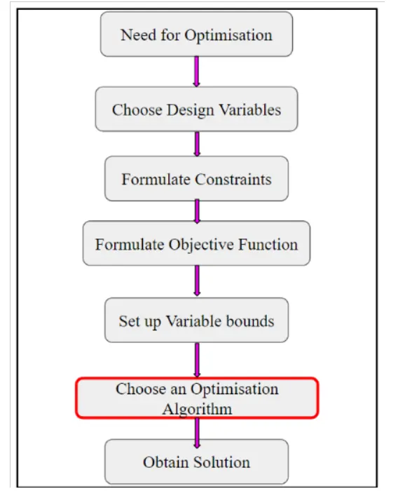
Here in the block representing the 'choose an optimization algorithm I have considered the genetic algorithm.

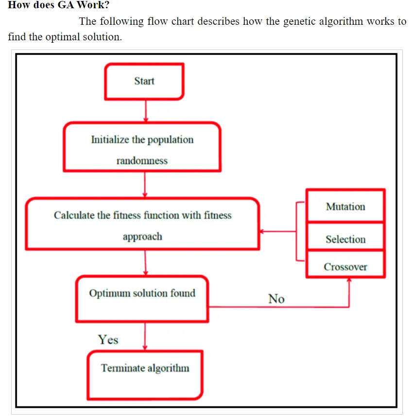
Genetic Algorithm: It is given with a command 'ga' in the Matlab. It is a search based optimization technique that uses genetics and natural selection as a process criteria to narrow down the optimal or near-optimal solution. It is also the most common algorithm used for the optimization technique.

The below flow diagram gives the bird's view on the process of the genetic algorithm. In Matlab, the genetic algorithm is an inbuilt command.

Code:

Case 1: Code just to figure out the global maxima

clear all
close all
clc

%inputs for the variables in 1D
x = linspace(0,0.6,150);
y = linspace(0,0.6,150);

%inputs conversion in 2D
[X Y] = meshgrid(x,y);

% to generate stalagmite function
for i = 1:length(X);
    for j = 1:length(Y);
        input_vector(1) = X(i,j);
        input_vector(2) = Y(i,j);
        f(i,j) = stalagmite(input_vector);
    end
end

surfc(X,Y,-f)
xlabel ('X')
ylabel ('Y')
shading interp

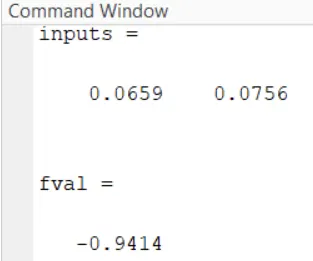
[inputs,fval] = ga(@stalagmite,2)  

Explanation:

1. The input for the required to solve this stalagmite function is two variables x and y (as we can see in the equation explained in the theory part).

Here the input for x and y is defined as '0 to 0.6' with a fixed interval of 150 times. This a 1D array.

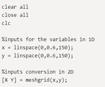
The command 'meshgrid' used in the Matlab is to convert the 1D to 2D array.

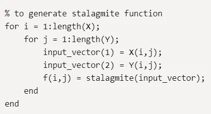
2. 'for loop' command is created with the variables i and j from the x and y respectively. With this, the value for the 'input_vector' is determined. stalagmite is a function for the coding is shown below. The output variable for the stalagmite is given as f(i,j) (as the inputs of x and y also depend on the i and j value)

Stalagmite function code:

function [F] = stalagmite(input_vector)
x = input_vector(1);
y = input_vector(2);
F1x = (sin(5.1*pi*x + 0.5)).^6;
F1y = (sin(5.1*pi*y + 0.5)).^6;
F2x = exp(-4*log(2)*((x - 0.0667).^2/0.64));
F2y = exp(-4*log(2)*((y - 0.0667).^2/0.64));
F = -(F1x.*F2x.*F1y.*F2y);
end

Again from the input_vector, the values of x and y are taken. This is subsequently fed into the stalagmite function.

The reason why the final F variable is given as negative is that the genetic algorithm is intended to find the minimum value from the initially assigned function. By assigning the negative value we are inversing the diagram which helps to determine the global maximum using the genetic algorithm.

3. Here the command 'surfc' creates a 3-dimensional surface plot with a contour plot underneath.

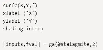
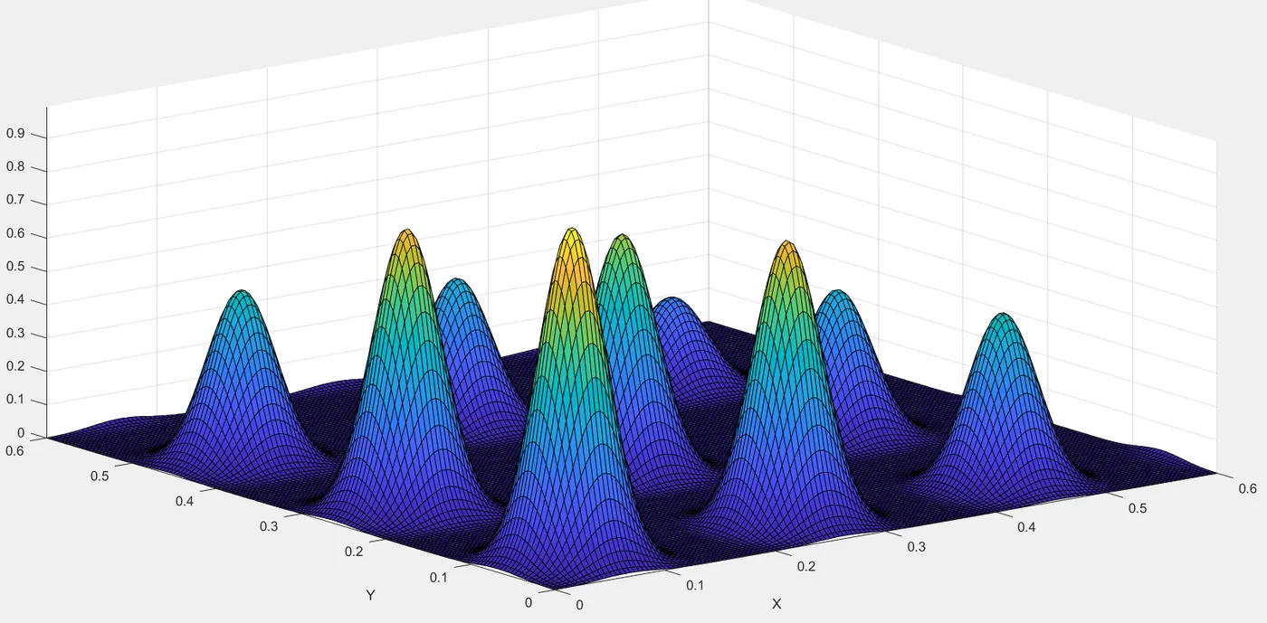
The command 'shading interp' is used to color fill the output instead of the mesh structure.

If the shading interp was removed, the resulting graph will be like the image shown below

4. finally the output array of inputs and fval(global maxima) is assigned to the 'ga' (genetic algorithm) of the stalagmite function. Here the '@' is the function handle and 2 is the number of variables.

Results for case 1:

1. The graph for the global maxima using the genetic algorithm coding is shown below,

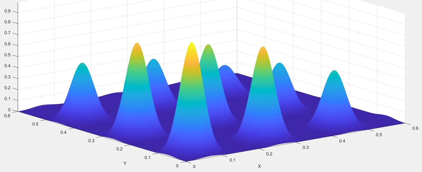
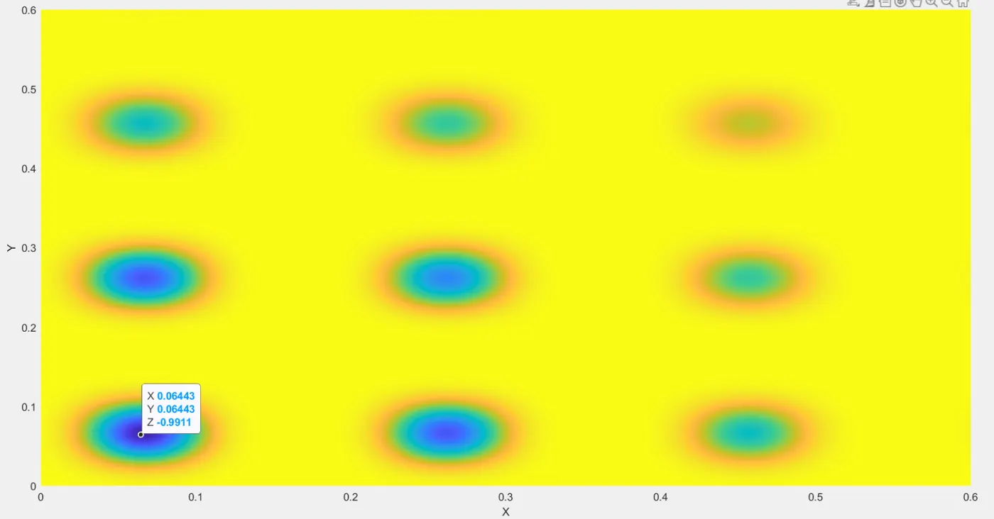
2. The result for the global maxima for this code is shown here this supported by the values taken via the 2D contour.

Case 2: Code just to determine the global maxima using statistical behavior/upper & lower bounds/ optimal solutions

clear all
close all
clc

%inputs for the variables in 1D
x = linspace(0,0.6,150);
y = linspace(0,0.6,150);
num_cases = 50;

%inputs conversion in 2D
[X Y] = meshgrid(x,y);

% to generate stalagmite function
for i = 1:length(X);
    for j = 1:length(Y);
        input_vector(1) = X(i,j);
        input_vector(2) = Y(i,j);
        f(i,j) = stalagmite(input_vector);
    end
end

[inputs,fval] = ga(@stalagmite,2)

% to identify the statistical behaviour 
tic
for i = 1:num_cases;
   [results,fopt(i)] = ga(@stalagmite,2);
   xopt(i) = results(1);
   yopt(i) = results(2);
end
study_time1 = toc

%plotting for the statistical behaviour
figure(1)
subplot(2,1,1)
hold on
surfc(X,Y,-f)
shading interp
plot3(xopt,yopt,-fopt,'marker','o','markersize',10,'markerfacecolor','r')
subplot(2,1,2)
plot(yopt)
hold off
xlabel('iterations')
ylabel('globalmaximum')
title('unconstrained limits')

% to identify the statistical behaviour 
tic
for i = 1:num_cases;
   [results,fopt(i)] = ga(@stalagmite,2);
   xopt(i) = results(1);
   yopt(i) = results(2);
end
study_time1 = toc

%plotting for the statistical behaviour
figure(1)
subplot(2,1,1)
hold on
surfc(X,Y,-f)
shading interp
plot3(xopt,yopt,-fopt,'marker','o','markersize',10,'markerfacecolor','r')
subplot(2,1,2)
plot(yopt)
hold off
xlabel('iterations')
ylabel('globalmaximum')
title('unconstrained limits')

% to identify the statistical behaviour 
tic
for i = 1:num_cases;
   [results,fopt(i)] = ga(@stalagmite,2);
   xopt(i) = results(1);
   yopt(i) = results(2);
end
study_time1 = toc

%plotting for the statistical behaviour
figure(1)
subplot(2,1,1)
hold on
surfc(X,Y,-f)
shading interp
plot3(xopt,yopt,-fopt,'marker','o','markersize',10,'markerfacecolor','r')
subplot(2,1,2)
plot(yopt)
hold off
xlabel('iterations')
ylabel('globalmaximum')
title('unbounded')

% to identify the stalagamite with upper and lower bounds
tic
for i = 1:num_cases;
   [results,fopt(i)] = ga(@stalagmite,2,[],[],[],[],[0,0],[1,1]);
   xopt(i) = results(1);
   yopt(i) = results(2);
end
study_time1 = toc

%plotting for the global maxima with upper and lower bounds
figure(2)
subplot(2,1,1)
hold on
surfc(X,Y,-f)
shading interp
plot3(xopt,yopt,-fopt,'marker','o','markersize',10,'markerfacecolor','r')
subplot(2,1,2)
plot(yopt)
hold off
xlabel('iterations')
ylabel('globalmaximum')
title('bounded')

% to identify the stalagamite with optim command
options = optimoptions('ga','populationsize',350)
tic
for i = 1:num_cases;
   [results,fopt(i)] = ga(@stalagmite,2,[],[],[],[],[0,0],[1,1],[],[],options);
   xopt(i) = results(1);
   yopt(i) = results(2);
end
study_time1 = toc

%plotting for the global maxima with the population limits
figure(3)
subplot(2,1,1)
hold on
surfc(X,Y,-f)
shading interp
plot3(xopt,yopt,-fopt,'marker','o','markersize',10,'markerfacecolor','r')
subplot(2,1,2)
plot(yopt)
hold off
xlabel('iterations')
ylabel('globalmaximum')
title('bounded')

Explanation of the code:

a) Using the previous Matlab code, the global maxima value kept on varying since the pool considered for the iterations was higher. To avoid that I have tried the Matlab coding in 3 different formats, the first one is "Statistical behavior".

To give a constraint on the iteration to be performed, I have assigned the value 50 for the number of cases.

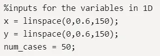
Here the inputs of x,y,stalagmite function is retained the same. The only change I have done is by limiting the value of i with to 50 values (number of cases).

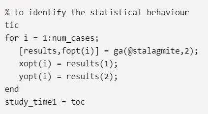
using this the values of xopt,yopt and fopt are determined. The command "tic and toc" is given to understand the duration for the code execution.

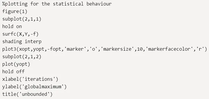
"figure(1)" is given because the subsequent two conditions are going to be plotted in the "figure(2) & figure(3)" "subplot" command is given to show 2 graphs on the same figure.

"plot3" is given as it helps plot the coordinates in the 3D space. The marker command is used to give the circle points on the graph. The size and color are also determined using the command.

in the second sub-plot, I plotting just the yopt (on y axis) and number of iterations (on x axis)

Results of the statistical behavior:

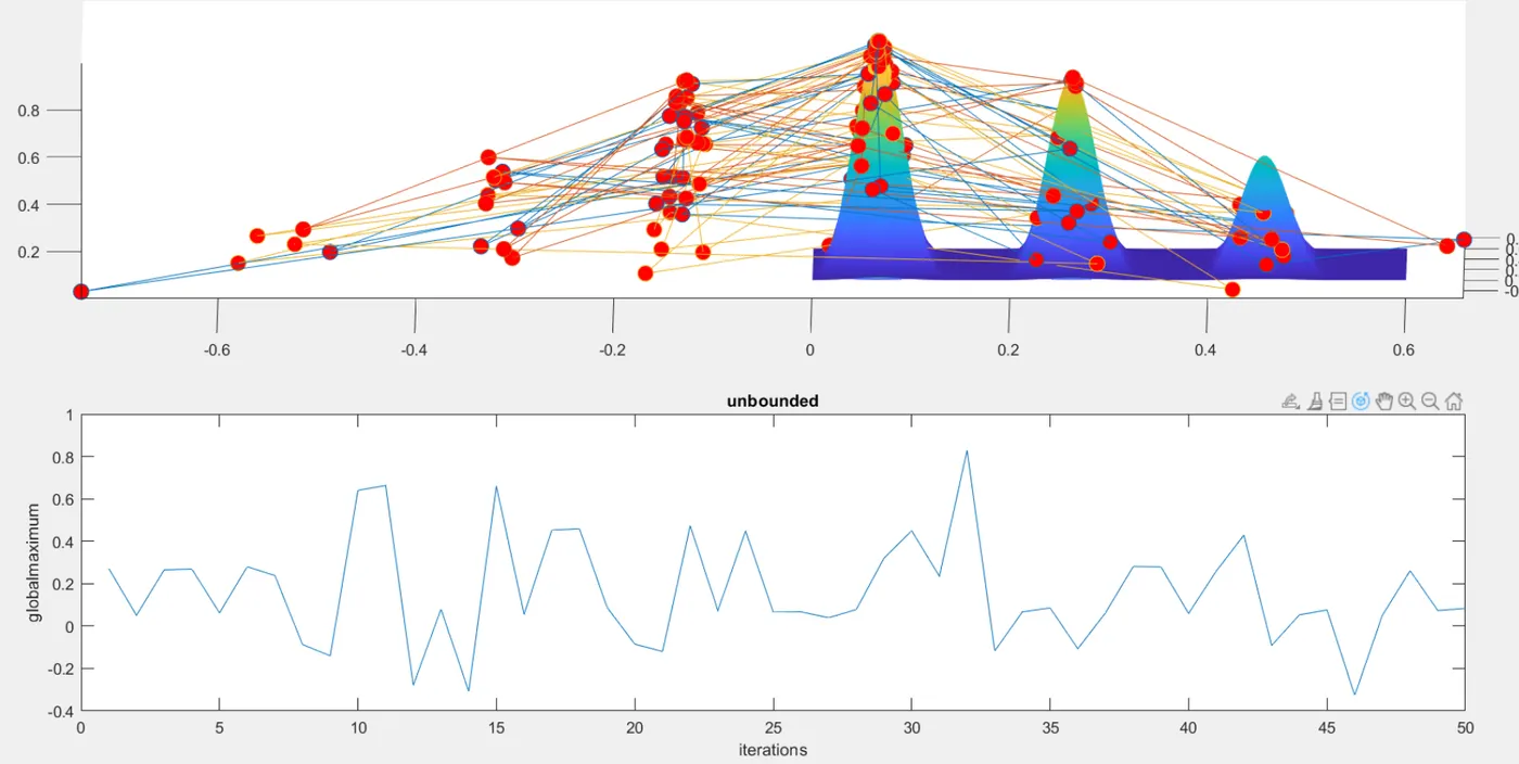
This is still not a feasible output because the genetic algorithm here predicts the multiple global maxima in the simulated graph.

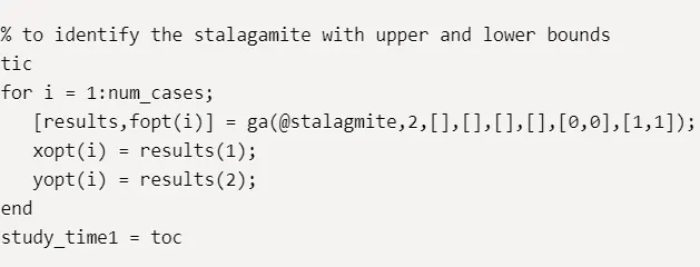
Explanation of the code for the upper and lower bound:

changed only in the genetic algorithm function. I have explained the symbols coming within the genetic algorithm

@ - function handle

stalagmite - function

first two [] [] - linear inequalities

next two [] [] - linear equalities

[0,0] - x and y values lower bound

[1,1] - x and y values upper bound

Results of the Upper and Lower Bound:

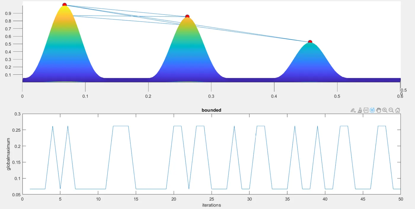
The variations are reduced to a certain extent when compared to the previous one, this is because the upper and lower bound values are assigned.

Explanation of the code for optimization command:

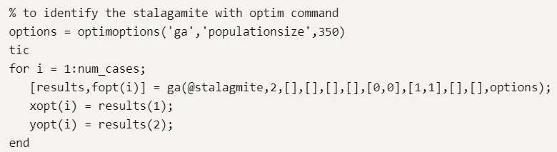
By default, the population size (random sampling) inbuilt within the genetic algorithm is 50 for a variable (x/y). If the sampling size is less the coding will help us to determine the local maxima instead of global maxima.

Hence using the inbulit command "optimoptions" I have increased the population size to 350.

I have explained the symbols coming within the genetic algorithm

@ - function handle

stalagmite - function

first two [] [] - linear inequalities

next two [] [] - linear equalities

[0,0] - x and y values lower bound

[1,1] - x and y values upper bound

[] - non linear constraints

[] - integer constants

This is followed by the usual plot commands.

Results of the optimization command:

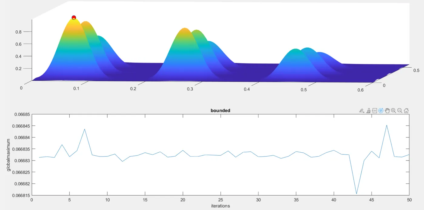
Thus by increasing the population size we were able to determine the optimal global maxima. This is followed by the usual plot commands.

Conclusion:

I found a method to optimize the stalagmite function using the genetic algorithm. In which i have used the 3 different methods to bring in the results, the later part by increasing the population size we have determined the global maxima.