Week 3 - Solving second order ODEs

Objective: To write a Matlab code to resolve the following simple pendulum equation,

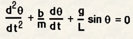
and to generate an animation for the same.

Theory:

As explained in the question part, the Simple pendulum motion depends upon Newton's second law of motion, F=ma. The above-mentioned equation will arrive if the derivation is done using second-order differential equation.

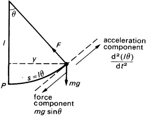
Code:

Main code:

clear all
close all
clc

% Inputs
g = 9.81;
l = 1;
m = 1;
b = 0.05;

% Initial condition
dis_vel = [0;3];

%time span
time_interval = linspace(0,20,500);

% solving the ODE
[t,x] = ode45(@(t,theta) ode_func(t,theta,g,l,m,b),time_interval,dis_vel);

%plotting 
figure (1)
hold on
subplot(2,1,1)
plot(t,x(:,1))
xlabel('Time')
ylabel('Angular displacement')
grid on
subplot(2,1,2)
plot(t,x(:,2))
xlabel('Time')
ylabel('Angular velocity')
grid on
ct=1;
theta = x(:,1);
for i = 1:length(theta);
    THETA = theta(i);
    x0 = 0;
    y0 = 0;
    x1 = l*sin(THETA);
    y1 = -l*cos(THETA);
    
    %plotting of the pendulum
    figure (2)
    %free end of the pendulum
    plot ([x0 x1],[y0 y1],'color','b','linewidth',2)
    hold on
    %bob
    plot (x1,y1,'Marker','o','Markersize',15,'MarkerFacecolor','r','MarkerEdgeColor','b')
    %fixed end of the pendulam
    plot ([-0.5 0.5],[0 0],'color','g','linewidth',4)
    hold off
    axis([-1.5 1.5 -1.5 1.5])
    M(ct) = getframe(gcf);
    ct = ct+1;
end
movie(M)
videofile = VideoWriter('Pendulum.avi','Uncompressed AVI');
open(videofile)
writeVideo(videofile,M)
close(videofile)

Function code:

function [dtheta_dt] = ode_func(t,theta,g,l,m,b)
theta1 = theta(1)
theta2 = theta(2)
dtheta1_dt = theta2;
dtheta2_dt = (-(b/m)*theta2) - ((g/l)*sin(theta1));
dtheta_dt = [dtheta1_dt; dtheta2_dt];
end

Code Explanation:

1. I have assigned the following inputs based on the data given in the problem statement. Here,'

g' is the acceleration due to gravity m/s^2

'l' is the length of the rope

'm' is mass of the bob

'b' is the damping coefficient

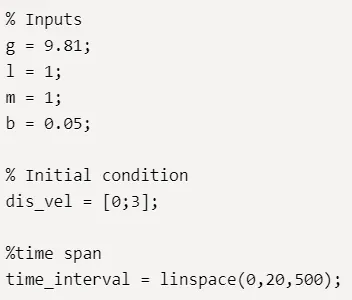
along with that, I have assigned a new variable as a matrix of initial angular displacement and angular velocity.

Since the time is varying from 0-20 sec, I gave the 'linspace' command to provide a fixed interval.

2. Since the equation given in the problem is in the differential equation. I used the command 'ode45', but this command in the Matlab is used to solve only first-order differential equations whereas in the given question the relation is in second-order differential equation form.

So to solve it we need to integrate it and solve like Runge-Kutta method which is also an ODE solver provided the initial conditions are given.

here '@(t,theta)' are two unknown values that are considered as inputs for the equation followed. Here instead of the equation, I have provided the function term of simplifying the second-order equation.

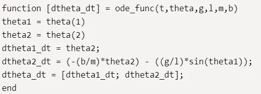
As we can see above, I assigned an array dtheta_dt as a function of the variables of time, angle, acceleration due to gravity, length of the string, the mass of the bob and the damping coefficient.

In the second-order differential equation, I assumed theta1 = theta(1) and dtheta1_dt = theta (2), thereby modifying the equation as dtheta2_dt = (-(b/m)*theta2) - ((g/l)*sin(theta1)).

Finally, the output variable dtheta_dt is a matrix of dtheta1_dt and dtheta2_dt.

3. After calculating the value of t and x, I have given the following command to plot a graph between angular velocity and time, angular displacement and time.

I have used the command 'subplot' to bring the two graphs separately yet in the same figure 1.

subplot(2,1,1) here 2 denotes 2 rows and 1 column and the last 1 represents the graph number, in this case, it's the first one.

x(:,1) indicates the displacement value obtained from the output.

'hold on' is given due to the usage of more than one plot in the command and 'grid on' is used to switch on the grids in the graph.

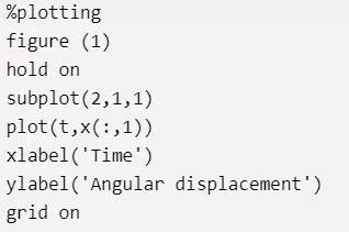
The same is followed for plotting time vs angular velocity.

4. To animate the simple pendulum based on the arrived values.

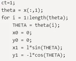
The command 'ct' is the counter, which is the frame depicting the graph of the first set of values.

Here I provided a variable containing the values of the angular displacement values that we arrived using the previous code.

To animate 'for' command is a must, for i = 1:length(theta) indicates the 1:total number of values.

This is followed by defining the coordinates, origin (x0,y0) = (0,0) and (x1,y1) =(l*sin(THETA)),-1*cos(THETA))

5. plotting for the animation,

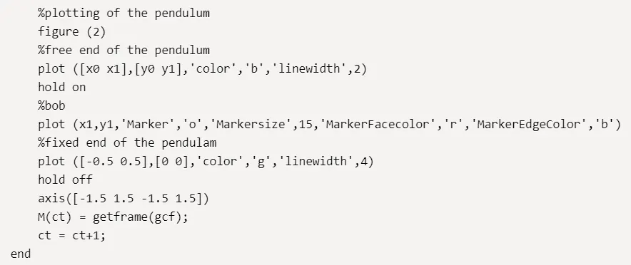
since this is going to be imprinted in the separate figure, I have given the command ' figure (2)'

The first plot is about the line connecting the bob and the origin.

The second plot is to create a bob at the end of the string, the coordinates at which the bob to created is mentioned in this case it is (x1,y1).

To create a circle, I gave 'Marker','o' (which is a circle) followed by defining its size and color. The circle can be created in the Matlab using the command 'viscircles' as well.

The third plot is about to create a line where the pendulum is fixed.

The command 'hold off' is so that any further plot will be recorded separately and it won't mix up with other graph.

To capture the Movie out of each counter, the command 'M(ct)=getframe(gcf)' is given, which is followed by the command 'ct = ct+1'for the continuous iteration.

Any for loop or function command it needs to end with the command 'end'.

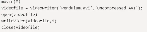
6. Finally to get the movie the below codes were used,

Error's occurred:

1. Multiple images were created during the animation, this occurred because I gave the 'hold on' command before even plotting the pendulum position. Later I placed the 'hold on' command after plotting the pendulum position which is resulted in correct animation.

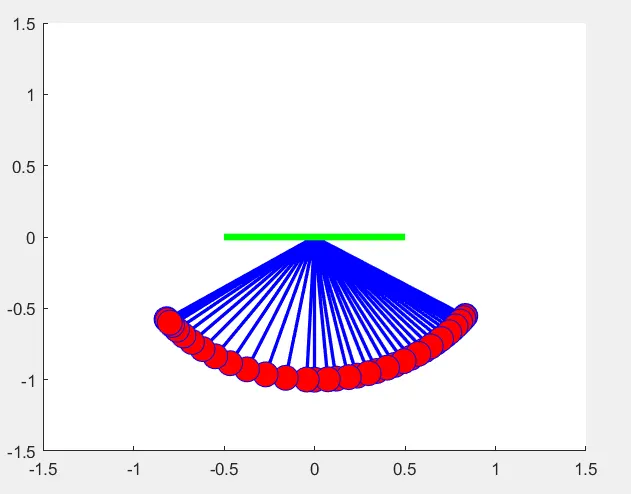
2. Here I received an error while defining the axis. Later figured out in the previous command I have defined the coordinates starting with the negative value whereas in the axis I started with the positive coordinate. This was later sorted out in the final code.

Result:

The animation video file of the simple pendulum can be found in the below link,

https://www.youtube.com/watch?v=37DAKQXjFbQ

Thus similar to Range-Kutta method in the mathematical model, we can breakdown and solve the second-order differential equation in the Matlab ODE45 command.