Project 1 - Parsing NASA thermodynamic data

Objective: To parse the NASA thermodynamic data which contains about 53 species and their coefficients. Using the file parsing technique in Matlab values of Cp,H and S need to calculated for each species. the formula for calculating mentioned variables are shown below,

Theory:

File parsing is a technique through which the input data is broken into desirable sequences and incorporate in the code to generate the required results. In this case, we have to calculate Enthalpy, Entropy and Specific heat.

Code:

This is the main code for determining the Cp, H and S.

clear all
close all
clc

A = fopen('THERMO.dat','r')
header = fgetl(A)
global_temp = fscanf(A,'%f')

% ignoring the comments
fgetl(A)
fgetl(A)
fgetl(A)

% species consolidation total 53 in the given NASA input
for i = 1:53;
sp = fgetl(A)
species_name = (sp(1:6))
coef1 = fgetl(A)
Ln_1 = strfind(coef1,'E')
c1 = str2num(coef1(1:(Ln_1(1)+3)))
c2 = str2num(coef1(Ln_1(1)+4:Ln_1(2)+3))
%c3 = coef1((27+4):(42+3))
c3 = str2num(coef1((Ln_1(2)+4):(Ln_1(3)+3)))
%c4 = coef1((42+4):(57+3))
c4 = str2num(coef1((Ln_1(3)+4):(Ln_1(4)+3)))
%c5 = coef1((57+5):(72+3))
c5 = str2num(coef1((Ln_1(4)+4):(Ln_1(5)+3)))

coef2 = fgetl(A)
Ln_2 = strfind(coef2,'E')
%c6 = coef2(1:12+3)
c6 = str2num(coef2(1:(Ln_2(1)+3)))
c7 = str2num(coef2(Ln_2(1)+4:Ln_2(2)+3))
c8 = str2num(coef2(Ln_2(2)+4:Ln_2(3)+3))
c9 = str2num(coef2(Ln_2(3)+4:Ln_2(4)+3))
c10 = str2num(coef2(Ln_2(4)+4:Ln_2(5)+3))

coef3 = fgetl(A)
Ln_3 = strfind(coef3,'E')
c11 = str2num(coef3(1:(Ln_3(1)+3)))
c12 = str2num(coef3(Ln_3(1)+4:Ln_3(2)+3))
c13 = str2num(coef3(Ln_3(2)+4:Ln_3(3)+3))
c14 = str2num(coef2(Ln_2(3)+4:Ln_2(4)+3))

% calculating the Specific heat, Enthalpy and Entropy
B = strfind(sp,'.');
L_t = str2num(sp((B(1)-3):(B(1)+3)));
H_t = str2num(sp((B(2)-3):(B(2)+3)));
t = linspace(L_t,H_t,100);
mid_t = 1000;
[Cp H S] = polynomials(c1,c2,c3,c4,c5,c6,c7,c8,c9,c10,c11,c12,c13,c14,t,mid_t)

mkdir('C:\Users\GANESHRAJ\OneDrive\Documents\MATLAB\Species\',species_name)

%plotting
% plot between cp vs local high and low temp of the species
figure(1)
plot(t,Cp,'linewidth',3)
xlabel('Temperature K')
ylabel('Cp KJ/kmol')
title(species_name)

figure(2)
plot(t,H,'linewidth',3)
xlabel('Temperature K')
ylabel('Enthalpy KJ/kmol')
title(species_name)

figure(3)
plot(t,S,'linewidth',3)
xlabel('High temperature K')
ylabel('Entropy KJ/kmol')
title(species_name)

program =(['C:\Users\GANESHRAJ\OneDrive\Documents\MATLAB\Species\',species_name])
cd(program)

%saving the plots
saveas(1,'Temperature vs Cp.jpg')
saveas(2,'Temperature vs Enthalpy.jpg')
saveas(3,'Temperature vs Entropy.jpg')

MWt = mol_weight(species_name);
F = fopen('Molecular weight of the species','w')
fprintf(F,'Species name   Molecular weight \n');
fprintf(F,'%s %f',species_name,MWt);
fclose(F)

cd('C:\Users\GANESHRAJ\OneDrive\Documents\MATLAB\') % returing back to the original directory 
end
fclose(A)

Code Explanation:

1. First, in order to access the input file, it has to be stored in the Matlab default directory. The path can be traced the path by typing the command "pwd" in the command section. The "fopen" command is used to open the input file and followed by that I have used "r" which means to read the input data.

Using the command "fgetl" to read the data from the input file line by line. Each "fgetl" command illustrates that the successive lines are incorporated in the code.

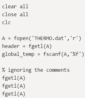
The first line is named as the header. This is followed by the command "fscanf" to read the numerical values form the input (those are values for global temperature), "%f" is used to read/write the numerical values. The next 3 lines in the input are only comments which are not required for obtaining the data. Hence without assigning any output variable the "fgetl" command is used thrice.

2. Since there are 53 species are mentioned in the input data file. So in order to perform the iteration 53 times, I have used i = 1:53. Now the first line of the species (which is monoatomic oxygen) is extracted using the "fgetl" command. To identify the species in the input, I have given the command sp(1:6), this 1:6 means the first 6 characters in the line command represents the species. I chose 6 since the maximum character of the species goes still 6.

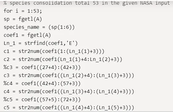
After the species line, there are 3 consecutive lines containing the values of 14 coefficients (for each species). In the first line, it has 5 coefficients. I extracted the values of 5 coefficients in the output named Ln_1 using the fgetl command. Then I used the command "strfind" which find the indicated the string position within the input file. This is followed by the delimiter "E" which clearly shows the number indicating the place where E is associated with the line as shown below,

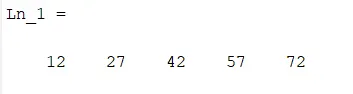
To extract the value of the one coefficient, using the command "str2num" and the number of the E shown above. The unique values of the coefficients are obtained as c1 to c14 for one species. In this way, all the values of coefficients are extracted.

3. Since in the question it is specifically mentioned to plot the graphs with respect to the global temperature and local temperature. Using the same logic of the command "strfind" , "." (as the delimiter), "str2num" I extracted the local low temperature and high temperature. In order to plot the values Cp,H and S with respect to the temperature we need a range of values for which the command "linspace" to obtain the temperature values within the fixed command interval.

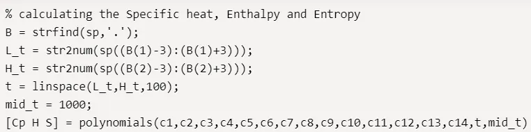
To calculate the values of Cp H and S I have used the "function" command.

The code for the function :

function [Cp H S] = polynomials(c1,c2,c3,c4,c5,c6,c7,c8,c9,c10,c11,c12,c13,c14,t,mid_t)
R = 8.314 % universal gas constant
for i = 1:length(t)
if t(i) > mid_t
    Cp = (c1+c2.*t+(c3.*t.^2)+(c4.*t.^3)+(c5.*t.^4)).*R;
    H = (c1+((c2.*t)./2)+((c3.*t.^2)./3)+((c4.*t.^3)./4)+((c5.*t.^4)./5)+(c6./t)).*R.*t;
    S1 = (c1.*log(t)+ c2.*t+((c3.*t.^2)./2)+((c4.*t.^3)./3)+((c5.*t.^4)./4)+c7).*R;
    else
    Cp = (c8+c9.*t+(c10.*t.^2)+(c11.*t.^3)+(c12.*t.^4)).*R;
    H = (c8+((c9.*t)./2)+((c10.*t.^2)./3)+((c11.*t.^3)./4)+((c12.*t.^4)./5)+(c13./t)).*R.*t;
    S = (c8*log(t)+ c9.*t+((c10.*t.^2)./2)+((c11.*t.^3)./3)+((c12.*t.^4)./4)+c14).*R;
end
end
end

The value of the local middle temperature is assigned as 1000 (based on the input). Now as per the question first 7 coefficients should be multiplied with the local high temperature and next 7 with the local low temperature.

Hence the command "if" is used that only if the temperature is above the 1000 K, the high-temperature range values of t get multiplied with the polynomials else the low-temperature range values are used.

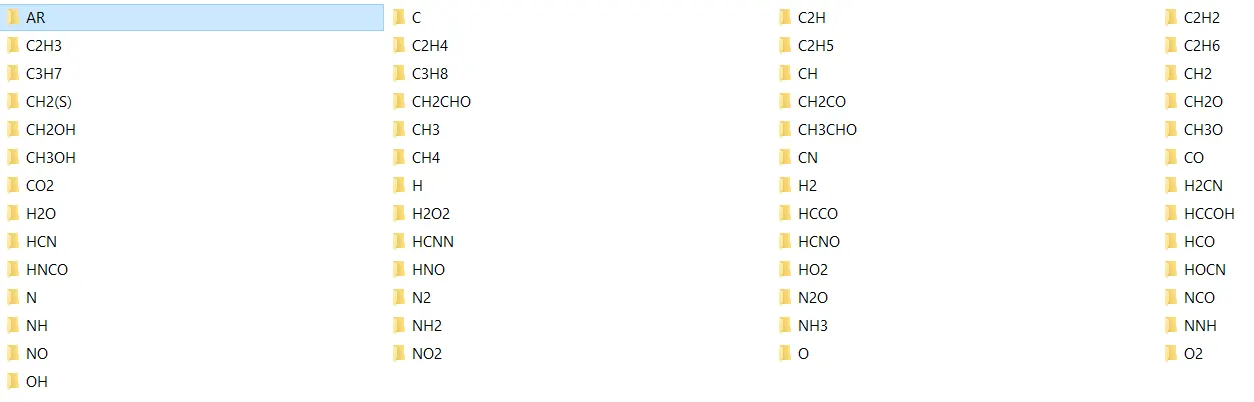
4. Now before plotting, it was clearly stated in the question that the results of the graph and the molecular weight of the species need to be documented in a separate folder structure automatically (ie., by coding). To initiate this, I gave the command "mkdir" following the path where the folder needs to be created. Since a new folder has to be created each individual species the command ends with the output variable "species_name".

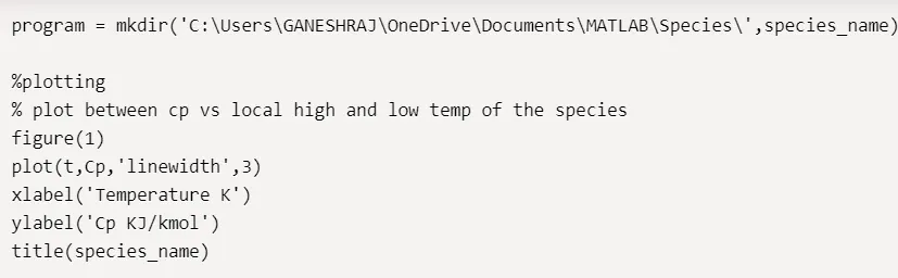
This is followed again by the conventional commands for plotting "plot,xlabel,ylabel and title". The command figure (1) is given as it is one among the 3 graphs that need to be generated for a species. Similarly, the same logic is applied to calculate the rest 2 graphs.

5. Now that we have created a new folder using the command "mkdir". We need to ensure that all the values generated are stored in that same folder. For that, we are referring to the path given for mkdir under the output program. This is then stored as a function of the command "cd" which is an inbuilt command in Matlab that modifies the path where the results of the Matlab are stored.

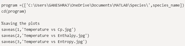
Then the command "saveas" is used to store the images of the 3 plots.

6. To obtain the Molecular weight of each species I have used the "function" command again.

Function code:

function MWt = mol_weight(species_name)
C = ['H','C','O','N','R','S'];
Atomic_weight = [1 12 16 14 40 32];
MW1 = 0;
for i = 1:length(species_name)
  for j = 1:length(C);  
if strcmp(species_name(i),C(j))
    MWt = MW1 + Atomic_weight(j);
    dt = j;
end
  end
  n = str2num(species_name(i));
  if n>1
      MWt = MWt + (Atomic_weight(dt)*(n-1));
end
end
end

The input for this function command "species_name" is already calculated. The monoatomic elements through the species are involved which is separately indicated as row C. This is followed by the Atomic weight of the respective monoatomic elements.

The two "for" commands are used to indicate the length of the species name and the monoatomic elements. A ned command "strcmp" is used to compare the 2 strings mentioned within the command. If the strings are matched it will give a logical value 1 or else it will give 0. Based on this logic the MWt (molecular weight) is calculated. Till this point, the code will be only able to calculate the molecular weight of only the monoatomic elements.

To achieve the molecular weight for species perfectly I used command "str2num" for the species_name under the output variable n. I also used the command "if" so that if the n value goes beyond 2 then the Molecular weight is changed accordingly.

Mwt (new weight) = Mwt(obtained for monoatomic elements) + (Atomic weight *(n-1)) (this will be applicable depending on the values of n).

7. After obtaining the values of the Molecular weight. Those results need to be documented in the respective species folder. Hence here I used the command "fopen". Unless at the early start of the code "r" (which was meant to read) here I used the command "w" which means the values are written in the file.

I used the command "fprintf" twice, in the first is just to write the headings of the obtained values which followed by the symbol "\n" this avoids the results to get clustered in a single column. The second "fprintf" is used to enter the obtained values, for species_name I have used the command "%s" (since the output is a character) "%f" (floating number) to capture the Molecular weight. This is closed by the command "fclose".

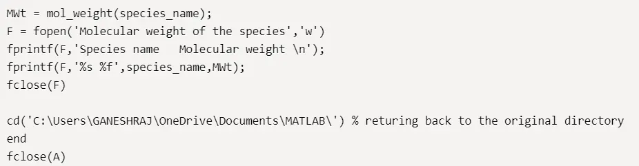
Finally, the "cd" command is set to its default location. This because we need to close the input data file which is actually placed in the default location.

Results:

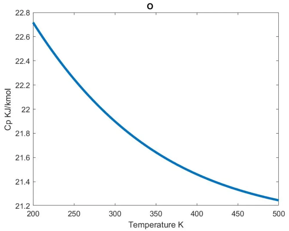
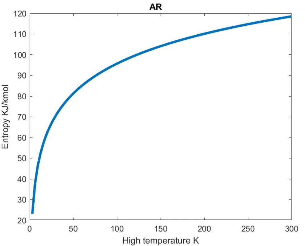
1. Plots of Cp, H and S for monoatomic element O,

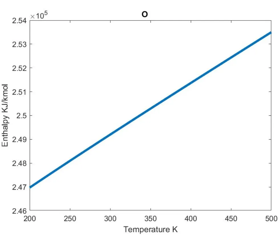
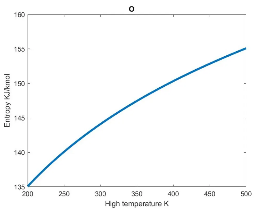
for elements AR,

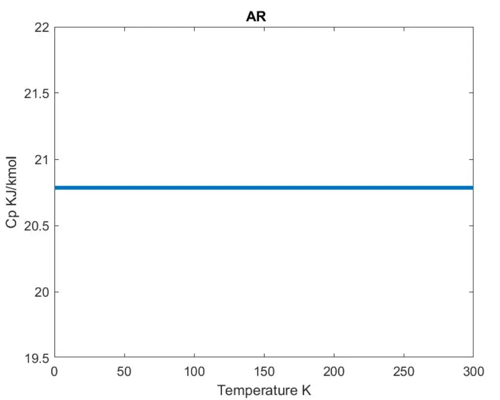
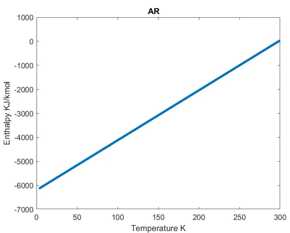
2. The folder location of the results of all the species,

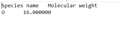
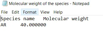
3. The Molecular weight of the species

Example 1: for monoatomic element O,

Example 2: for monoatomic element AR,

Conclusion:

I have learned how to parse the input file and incorporate the data's in the code, thus values of CP, H and S are determined with the polynomial equation given in the input.

References:

1. All the Matlab help section to understand the commands like "str2num", "str2double", "strfind","strcmp", "if", "while", "mkdir", "cd".

2. https://skill-lync.com/projects/nasa-file-parsing-79131 &https://skill-lync.com/projects/FILE-PARSING-98158 to understand the code flow and logic.