Week 4 - Genetic Algorithm

Aim: to optimize the given stalagmite function and find the global maxima of the function.

THEORY :

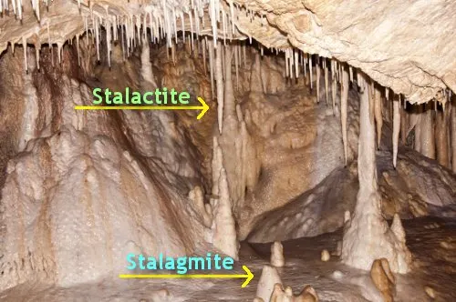
What is a stalagmite?

Stalactite and stalagmite, elongated forms of various minerals deposited from solution by slowly dripping water. A stalactite hangs like an icicle from the ceiling or sides of a cavern. A stalagmite appears like an inverted stalactite, rising from the floor of a cavern.

What is a genetic algorithm?

Genetic Algorithm (GA) is a search-based optimization technique based on the principles of Genetics and Natural Selection. It is frequently used to find optimal or near-optimal solutions to difficult problems that otherwise would take a lifetime to solve. It is frequently used to solve optimization problems, in research, and in machine learning.

Optimization:

Optimization is the process of making something better. In any process, we have a set of inputs and a set of outputs as shown in the following figure.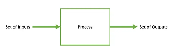

Optimization refers to finding the values of inputs in such a way that we get the “best” output values. The definition of “best” varies from problem to problem, but in mathematical terms, it refers to maximizing or minimizing one or more objective functions, by varying the input parameters.

The set of all possible solutions or values which the inputs can take make up the search space. In this search space, lies a point or a set of points which gives the optimal solution. The aim of optimization is to find that point or set of points in the search space.

Genetic algorithm:

Nature has always been a great source of inspiration to all mankind. Genetic Algorithms (GAs) are search based algorithms based on the concepts of natural selection and genetics. GAs are a subset of a much larger branch of computation known as Evolutionary Computation.

GAs were developed by John Holland and his students and colleagues at the University of Michigan, most notably David E. Goldberg and has since been tried on various optimization problems with a high degree of success.

In GAs, we have a pool or a population of possible solutions to the given problem. These solutions then undergo recombination and mutation (like in natural genetics), producing new children, and the process is repeated over various generations. Each individual (or candidate solution) is assigned a fitness value (based on its objective function value) and the fitter individuals are given a higher chance to mate and yield more “fitter” individuals. This is in line with the Darwinian Theory of “Survival of the Fittest”.

In this way, we keep “evolving” better individuals or solutions over generations, till we reach a stopping criterion.

Genetic Algorithms are sufficiently randomized in nature, but they perform much better than random local search (in which we just try various random solutions, keeping track of the best so far), as they exploit historical information as well.

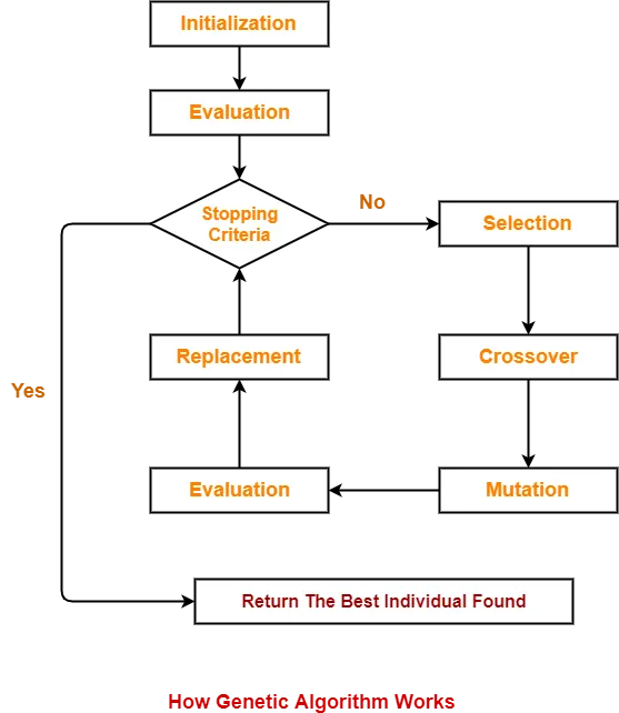
The flow chart for this is as follows:

Basic Terminology used:

Before beginning a discussion on Genetic Algorithms, it is essential to be familiar with some basic terminology that will be used throughout this tutorial.

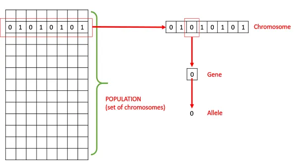
• Population − It is a subset of all the possible (encoded) solutions to the given problem. The population for a GA is analogous to the population for human beings except that instead of human beings, we have Candidate Solutions representing human beings.

• Chromosomes − A chromosome is one such solution to the given problem.

• Gene − A gene is one element position of a chromosome.

• Allele − It is the value a gene takes for a particular chromosome.

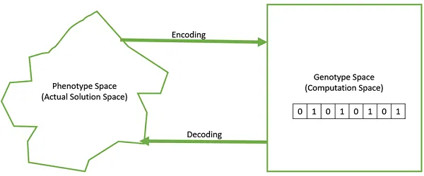
• Genotype − Genotype is the population in the computation space. In the computation space, the solutions are represented in a way that can be easily understood and manipulated using a computing system.

• Phenotype − Phenotype is the population in the actual real-world solution space in which solutions are represented in a way they are represented in real-world situations.

• Decoding and Encoding − For simple problems, the phenotype and genotype spaces are the same. However, in most of the cases, the phenotype and genotype spaces are different. Decoding is a process of transforming a solution from the genotype to the phenotype space, while encoding is a process of transforming from the phenotype to genotype space. Decoding should be fast as it is carried out repeatedly in a GA during the fitness value calculation.

  For example, consider the 0/1 Knapsack Problem. The Phenotype space consists of solutions that just contain the item numbers of the items to be picked.

  However, in the genotype space, it can be represented as a binary string of length n (where n is the number of items). A 0 at position x represents that x^th item is picked while a 1 represents the reverse. This is a case where genotype and phenotype spaces are different.

• Fitness Function − A fitness function simply defined is a function that takes the solution as input and produces the suitability of the solution as the output. In some cases, the fitness function and the objective function may be the same, while in others it might be different based on the problem.

• Genetic Operators − These alter the genetic composition of the offspring. These include crossover, mutation, selection, etc.

Working of the algorithm:

• Initialize the population. This can be done in two ways:

1. Random initialization
2. Heuristic initialization

• Evaluates the fitness of the population.
• If the fitness function is satisfied then terminate and give the results.
• If not then select the best fitness values.
• Make a crossover and mutate and evaluate them again according to the fitness function and replace the existing values.
• If the stopping criteria are met terminate or else continue the iterations until the best value is obtained.

=>The termination condition of a Genetic Algorithm is important in determining when a GA run will end. It has been observed that initially, the GA progresses very fast with better solutions coming in every few iterations, but this tends to saturate in the later stages where the improvements are very small. We usually want a termination condition such that our solution is close to the optimal, at the end of the run.

Usually, we keep one of the following termination conditions −

• When there has been no improvement in the population for X iterations.
• When we reach an absolute number of generations.
• When the objective function value has reached a certain pre-defined value.

here we have used a fixed no. of iterations to find the best possible value.

GA SYNTAX

x = ga(fun,nvars)

Here it evaluates the function handle fun for the given input with nvars(no. of variables) and returns x as the local minimum value.

x = ga(fun,nvars,A,b,Aeq,beq,lb,ub)

Here it evaluates as the same way as above but with certain constraints as the upper and lower boundaries so as to minimize or restrict the search space.

x = ga(fun,nvars,A,b,Aeq,beq,lb,ub,nonlcon,options)

Here it evaluates the function handle with the constraints and restrictions by other values of options which can be defined by optimoptions.

CODE:

clear all
close all
clc
x = linspace(0,0.6,150);
y = linspace(0,0.6,150);
num_cases = 50;
%creating a 2D mesh
[xx yy] = meshgrid(x,y);

for i = 1:length(xx)
    for j = 1:length(yy)
        input_vector(1) = xx(i,j);
        input_vector(2) = yy(i,j);
        f(i,j) = stalagmite(input_vector);
    end
end
tic
%study 1 : statistical behaviour without bounds
for k = 1:num_cases
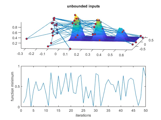
    [inputs_1,fopt_1(k)] = ga(@stalagmite,2);
    xopt_1(k) = inputs_1(1);
    yopt_1(k) = inputs_1(2);
end
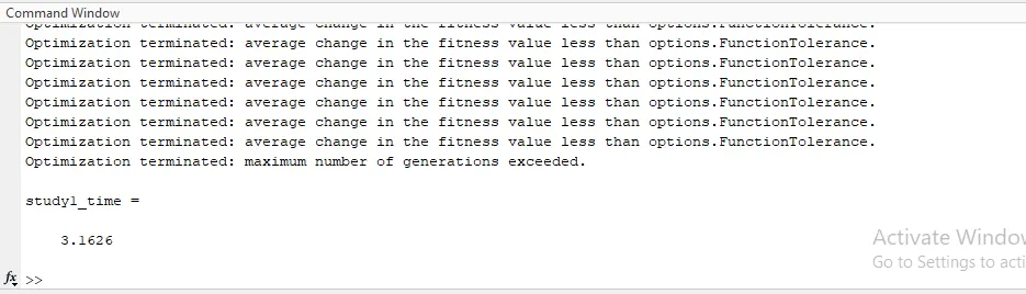
study1_time = toc
figure(1)
subplot(2,1,1)
hold on
surfc(xx,yy,-f)
shading interp
plot3(xopt_1,yopt_1,-fopt_1,'marker','o','markersize',5,'markerfacecolor','r')
title('unbounded inputs')
subplot(2,1,2)
plot(-fopt_1)
xlabel('iterations')
ylabel('function minimum')

%study 2 : statistical behaviour with lower and upper bounds
tic
for k = 1:num_cases
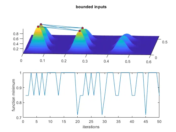
    [inputs_2,fopt_2(k)] = ga(@stalagmite,2,[],[],[],[],[0;0],[0.6;0.6]);
    xopt_2(k) = inputs_2(1);
    yopt_2(k) = inputs_2(2);
end
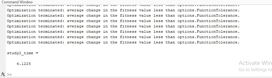
study2_time = toc

figure(2)
subplot(2,1,1)
hold on
surfc(xx,yy,-f)
shading interp
plot3(xopt_2,yopt_2,-fopt_2,'marker','o','markersize',5,'markerfacecolor','r')
title('bounded inputs')
subplot(2,1,2)
plot(-fopt_2)
xlabel('iterations')
ylabel('function minimum')

%study 3  increasing the number of ga iterations
options = optimoptions('ga')
options = optimoptions(options,'Populationsize',170);

tic
for k = 1:num_cases
    [inputs_3,fopt_3(k)] = ga(@stalagmite,2,[],[],[],[],[0;0],[0.1;0.1],[],[],options);
    xopt_3(k) = inputs_3(1);
    yopt_3(k) = inputs_3(2);
end
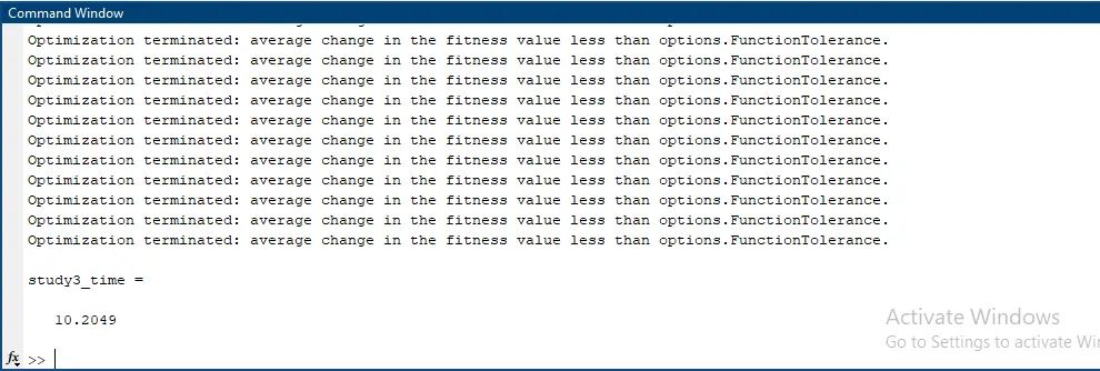
study3_time = toc
figure(3)
subplot(2,1,1)
hold on
surfc(xx,yy,-f)
shading interp
plot3(xopt_3,yopt_3,-fopt_3,'marker','o','markersize',5,'markerfacecolor','r')
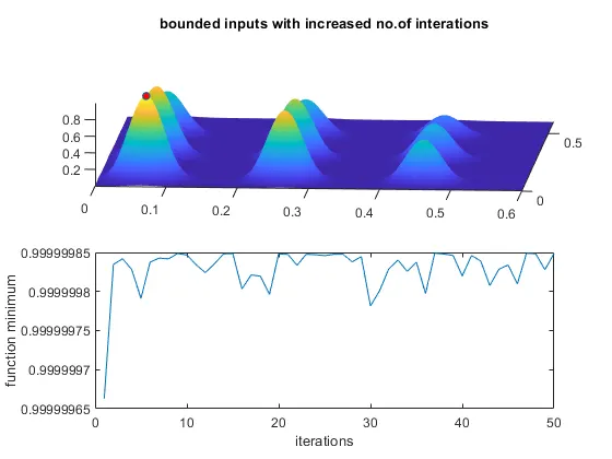
title('bounded inputs with increased no.of interations')
subplot(2,1,2)
plot(-fopt_3)
xlabel('iterations')
ylabel('function minimum')

    

function [F] = stalagmite(inputs)

x = inputs(1);
y = inputs(2);

f1 = (sin(5.1.*pi.*x+ 0.5)).^6;

f2 = (sin(5.1.*pi.*y+0.5)).^6;

f3 = exp((-4.*log(2).*(x-0.0667).^2)./(0.64));

f4 = exp((-4.*log(2).*(y-0.0667).^2)./(0.64));

[F] = -(f1.*f2.*f3.*f4);

end

Procedure:

Since the ga solver gives the local minimum as default I used a negative sign in the formula of stalagmite to maximize it. but as the plot was inverted I again used a negative sign to plot fopt to get a straight graph.

1.Define the stalagmite function according to the given formulae in a separate script.

2.Define the x and y values using linspace and form a meshgrid between them as [xx yy].

3.Use a for loop to evaluate the stalagmite function of different values of xx and yy.

4.Definfe num_cases and assign a value of 50. This is the no.of iterations for the ga.

5.I have used 3 study cases for evaluating and testing the ga.

6.In the first case I had run the ga code in a for loop 50 times without any bounds.

7.In this case it took random samples sometimes even beyond the maximum values of xx and yy.

8.So I used the 2nd case but this time I gave the lower and upper bounds for the ga function.

9. This helped in getting converged optimized values.

10.For converging the results furthermore and getting a more optimized result I used another syntax of ga and the upper and lower bounds and also the population size.

11.Thus I got a converged result of 2 optimized values.

RESULTS:

REFERENCES :

https://www.tutorialspoint.com/genetic_algorithms/genetic_algorithms_fundamentals.htm

https://in.mathworks.com/help/gads/ga.html

https://apacheignite.readme.io/v2.7.6/docs/genetic-algorithms

ERRORS:

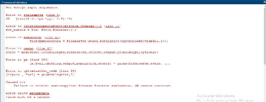
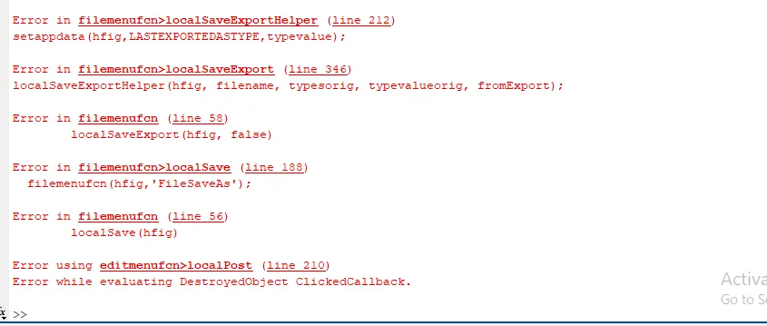
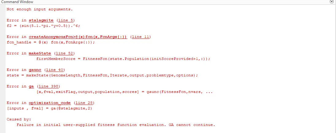
i was using two inputs for stalagmite function but the ga solver does not support that.

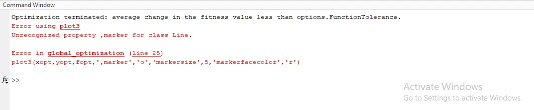
it is a typing error I typed ',marker'.