Week 3 - Solving second order ODEs

Objective:

To solve the ode for a simple pendulum and simulate its motion.

Problem Statement:

Write a program in Python that will simulate the pendulum motion.

Solution Procedure:

1. Import the required modules.(numpy, scipy, matplotlib, and math)
2. Define a function that returns an array dtheta_dt with the two odes. The second-order differential equation is solved using two single order differential equations.
3. Declare the variables, damping coefficient, acceleration due to gravity, length of the pendulum mass of the bob.
4. Now define the initial conditions for the displacement and velocity.
5. Also, declare the time span of oscillation.
6. Use odeint to solve the differential equations.
7. Plot the results on a graph.(displacement vs time & velocity vs time)
8. Specify the legends and axis limits.
9. Use a for loop between 1 and the length of t.
10. For the animation use a variable ct and increment it for every loop. Use ct to save the plots and later use the command prompt and image magic application to stitch the images to get a gif.

Code:

import numpy as np
from scipy.integrate import odeint
import matplotlib.pyplot as plt
import math
#function that returns dz/dt
def model(theta,t,b,g,l,m):
	theta1 = theta[0]
	theta2 = theta[1]
	dtheta1_dt = theta2
	dtheta2_dt = -(b/m)*theta2-(g/l)*math.sin(theta1)
	dtheta_dt = [dtheta1_dt,dtheta2_dt]
	return dtheta_dt
b = 0.02
g = 9.81
l = 1
m = 0.1
#intial conditions
theta_0 = [0,3]
#time points
t = np.linspace(0,20,150)
T = len(t)
#solve ODE
theta = odeint(model,theta_0,t,args=(b,g,l,m))
#plot results
plt.figure(1)
plt.plot(t,theta[:,0],'b-',label =r'$\frac{d\theta_1}{dt}=\theta2$')
plt.plot(t,theta[:,1],'r--',label =r'$\frac{d\theta2}{dt}=-\frac{b}{m}\theta_2-\frac{g}{l}sin\theta_1$')
plt.ylabel('Plot')
plt.xlabel('time')
plt.legend(loc='best')
plt.xlim([0,12])
plt.ylim([-5,5])
plt.show()
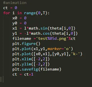
#animation
ct = 0
for i in range(0,T):
	x0 = 0
	y0 = 0
	x1 = l*math.sin(theta[i,0])
	y1 = -l*math.cos(theta[i,0])
	filename ='test%05d.png'%ct
	plt.figure()
	plt.plot(x1,y1,marker='o')
	plt.plot([x0,x1],[y0,y1],'k-')
	plt.xlim([-2,2])
	plt.ylim([-2,2])
	plt.savefig(filename)
	ct = ct+1

Results:

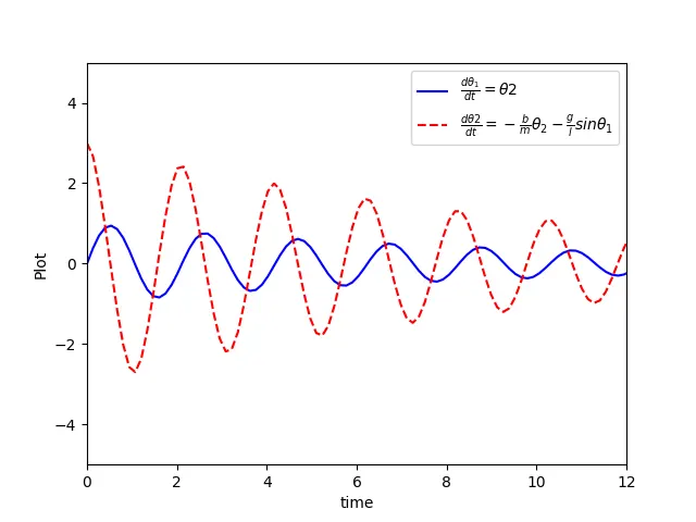
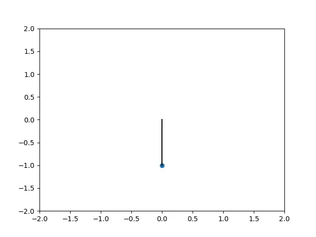
Errors:

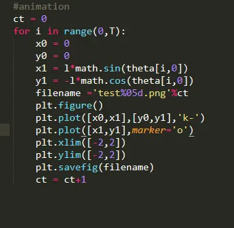
I did not define the marker position(x1,y1) correctly. Due to this the graph plot was shown as:

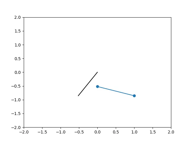
Then I corrected the syntax of defining the point to