Simulation of the motion of a Simple Pendulum

AIM: To solve the second-order ode to simulate the transient motion of a simple pendulum and create an animation of its motion.

GOVERNING EQUATIONS :

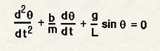
This equation is integrated using the ode solver to calculate the angular displacement given by `theta`

• Angular displacement : Angular displacement is defined as “the angle in radians (degrees, revolutions) through which a point or line has been rotated in a specified sense about a specified axis”.

SI units of angular displacement are Radian or Degrees.

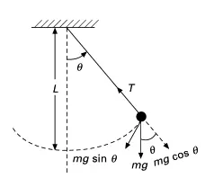
• Simple Pendulum: It is a mechanical system that moves in an oscillatory motion. It consists of a point mass 'm' suspended by means of a light inextensible string of length L from fixed support as shown in Fig.

The motion occurs in a vertical plane and is driven by a gravitational force. The forces which are acting on the mass are shown in the figure.

PROCEDURE:

• First, create a function to solve the second-order ode.
• To solve a second order ode we have to break it into two first-order odes.
• Here the two first-order odes are dtheta1_dt and dtheta2_dt.
• Assign them under theta as a solution vector.
• Now give all the inputs required(b,g,l,m, theta,span of integration i.e t values).
• Use the ode45 solver to solve the ode function that we created in a previous program.
• [t,y] = ode45(odefun,tspan,y0), where tspan = [t0 tf], integrates the system of differential equations y′=f(t,y) from t0 to tf with initial conditions y0. Each row in the solution array y corresponds to a value returned in a column vector t.
• Then plot the results theta1 and theta2 against t will give a plot of displacement vs time and velocity vs time.
• Now for the animation fix a point x0 and y0 as 0 and 0.
• Vary x1 and y1 according to the theta values obtained by solving the ode.
• Now use the marker command to create the ball.
• Finally, create a movie accordingly.

CODE :

clear all
close all
clc
%inputs
b=0.05;
m=1;
g=9.81;
l=1;
%intial conditions
theta=[0;3];
%time conditions
t_span=linspace(0,20,1000);
%solving the ode
[t,results]=ode45(@(t,theta) ode_func1(t,theta,b,g,l,m),t_span,theta);
%plotting
figure(1)
hold on
plot(t,results(:,1));
plot(t,results(:,2));
legend('time vs displacement','time vs velocity')
xlabel('plot')
ylabel('time')
%animation
l=0.5;
ct=1;
for i=1:length(t_span)
x0=0;
y0=0;
x1=l.*sin(results(i,1));
y1=-l.*cos(results(i,1));
figure(2)
plot([x0 x1],[y0 y1],'color','b','linewidth',3)
line([-0.3 0.3],[0 0],'linewidth',2,'color','k')
hold on
plot(x1,y1,'o','MarkerFaceColor','red','MarkerSize',15,'MarkerEdgeColor','red')
hold off
axis([-1 1 -1 1])
pause(0.03)
M(ct)=getframe(gcf);
ct=ct+1;
end
movie(M)
videofile=VideoWriter('simplependulum.avi','uncompressed AVI');
open(videofile)
writeVideo(videofile,M)
close(videofile)

THE FUNCTION:

function [dtheta_dt]=ode_func1(t,theta,b,g,l,m)
theta1=theta(1);
theta2=theta(2);
dtheta1_dt=theta2;
dtheta2_dt=((-b/m)*theta2)-((g/l)*sin(theta1));
dtheta_dt=[dtheta1_dt;dtheta2_dt];
end

Results:

Animation: https://youtu.be/DYSjZ9Dp4SY

Plots:

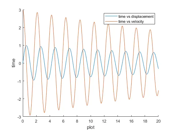
The red curve is for time vs velocity and blue curve is for time vs displacement.

Both the curves vary according to the damping factor b.

Errors:

I had made a mistake while defining the function which i corrected.

I have mistakenly saved the function program and main program in different folders.

I had made a mistake calling the ode function.

I had made a typing mistake here.