Week 4 - Curve fitting

AIM:To write a MATLAB code to plot a curve and compare it with original dataset.

OBJECTIVES:

• Write code to fit a linear and cubic polynomial for the Cp data.
• Plot the linear and cubic fit curves along with the raw data points. Title and axes labels are a must, legends could be shown if necessary.
• Write a code to show splitwise method.
• Explain the parameters used to measure the fitness characteristics for both the curves.

THEORY:

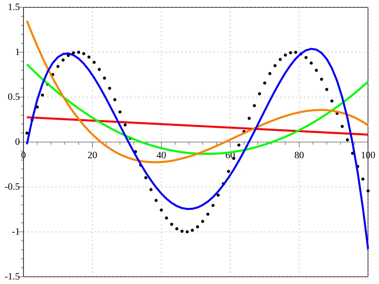
• Curve Fitting: Curve fitting is the process of constructing a curve , or mathematical function, that has the best fit to a series of data points, possibly subject to constraints. Curve fitting can involve either interpolation, where an exact fit to the data is required, or smoothing, in which a "smooth" function is constructed that approximately fits the data. A related topic is regression analysis, which focuses more on questions of statistical inference such as how much uncertainty is present in a curve that is fit to data observed with random errors. Fitted curves can be used as an aid for data visualization, to infer values of a function where no data are available, and to summarize the relationships among two or more variables. Extrapolation refers to the use of a fitted curve beyond the range of the observed data, and is subject to a degree of uncertainty since it may reflect the method used to construct the curve as much as it reflects the observed data.

• Fitting lines and polynomial functions to data points:

The first degree polynomial equation

is a line with slope a. A line will connect any two points, so a first degree polynomial equation is an exact fit through any two points with distinct x coordinates.

If the order of the equation is increased to a second degree polynomial, the following results:

This will exactly fit a simple curve to three points.

If the order of the equation is increased to a third degree polynomial, the following is obtained:

This will exactly fit four points.

A more general statement would be to say it will exactly fit four constraints. Each constraint can be a point, angle, or curvature (which is the reciprocal of the radius of an osculating circle).

MEASURING FITNESS CHARATERISTICS OF THE CURVES:

There are various methods to measure the fitness characteristics of the curve(s). Some of them are:

1. Sum of squares error (SSE)
2. Sum of squares regression (SSR)
3. Total sum of squares (TSS)
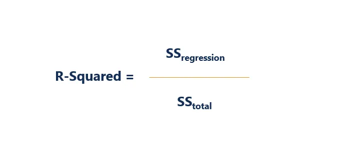
4. R squared (R²)

.....and many more

• SSE: SSE represents sum of squares error, also known as residual sum of squares. It is the difference between the observed value and the predicted value.Usually, the lower the sum of squares error better model the regression. SSE is that part of the total variation which is not modeled by the regression line.

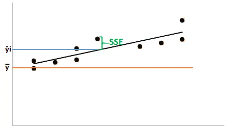
• y_i is the one of the value in the sample
• ŷ_i is the predicted value

• SSR:Sum of squares due to regression is represented by SSR. It is the difference between the predicted value and the sample mean.

  

  

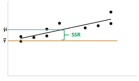
  • ŷ_i is the predicted value
  • y̅ is the sample mean

• TSS: TSS represents the total sum of squares. It is the squared values of the dependent variable to the sample mean. In other words, the total sum of squares measures the variation in a sample.

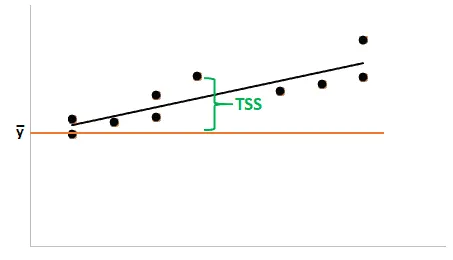
• ŷ_i is the predicted value
• y̅ is the sample mean

The relationship between TSS, SSR and SSE is mathematically represented by

TSS = SSR+SSE

• R Squared:R-Squared (R² or the coefficient of determination) is a statistical measure in a regression model that determines the proportion of variance in the dependent variable that can be explained by the independent variable. In other words, r-squared shows how well the data fit the regression model (the goodness of fit).

The most common interpretation of r-squared is how well the regression model explains observed data. For example, an r-squared of 60% reveals that 60% of the variability observed in the target variable is explained by the regression model. Generally, a higher r-squared indicates more variability is explained by the model.

Usually R squared value above 0.95 is considered as good fit.

• MATLAB Code(s):

1. Linear vs Cubic curve fitting:

%Curve fitting
clear all
close all
clc

%Preaparing Data
cp_data=load('data');
temp=cp_data(:,1); %K
cp=cp_data(:,2); %KJ/K-Kmol

%CURVE FITTING

%linear fit: cp=a*T+b
coeff_1=polyfit(temp, cp, 1);
predicted_cp_1=polyval(coeff_1, temp);

%cubic fit: cp=a*T^3 + b*T^2 + c*T + d
coeff_3=polyfit(temp, cp, 3);
predicted_cp_3=polyval(coeff_3, temp);

%Plotting
plot(temp,cp,LineWidth=2,Color=[1 0 0])
hold on
plot(temp,predicted_cp_1,LineWidth=2,Color=[0 1 0])
plot(temp,predicted_cp_3,LineWidth=2,Color=[0 0 1])
legend('Original Data', 'Linear Fit', 'Cubic Fit')
xlabel('Temperature [K]')
ylabel('Specific Heat [KJ/K-Kmol]')

EXPLANATION:

1. Under '%Preparing Data', we have used load command to load data from the file 'data', which is saved in the same directory of our MATLAB code.
2. The data file contains two columns, first one containing Temperatures, second containing the corresponding C_p values.
3. Assuming that the relationship between cp and temp is a polynomial in nature and in order to get the coeff.(s), the function that we are going to use is polyfit. It first takes the values of the independent variable from the sample, then the values of the dependent variable. The next value is the degree of the equation.
4. Once we get the coeff.(s), we calculate the predicted values using the temperature values from the sample using the function polyval.
5. Now, just by changing the degree in the polyfit function, we can get multiple polynomial relations.
6. Now, in order to compare the curves visually, we plot them in the same figure window.

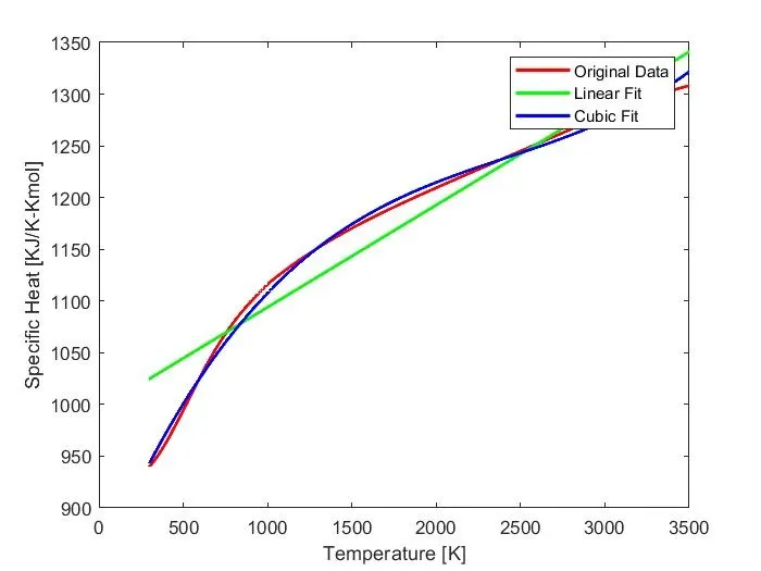
Thus, from the above figure, it is clear that the cubic curve fits much better than the linear curve.

2. To measure the fitness characteristics of the Curves:

%Curve Fittting 
%To measure the fitness characteristics of the Curves

%linear curve
error_1=(cp-predicted_cp_1);
avg_1=mean(error_1.^2);
SSE_1=sum(error_1.^2);

SSR_1=sum((predicted_cp_1 - mean(cp)).^2);

SST_1=SSR_1+SSE_1;

R_squared_1=SSR_1/SST_1;
R_squared_1_percentage=R_squared_1*100;

Linear_Character=table(avg_1, SSR_1, SSE_1, SST_1, R_squared_1_percentage);
Linear_Character.Properties.VariableNames={'ERROR', 'SSR', 'SSE', 'SST', 'R^2'};

%cubic fit

error_3=(cp-predicted_cp_3);
avg_3=mean(error_3.^2);
SSE_3=sum(error_3.^2);

SSR_3=sum((predicted_cp_3 - mean(cp)).^2);

SST_3=SSR_3+SSE_3;

R_squared_3=SSR_3/SST_3;
R_squared_3_percentage=R_squared_3*100;

Cubic_Character=table(avg_3,SSR_3,SSE_3,SST_3,R_squared_3_percentage);
Cubic_Character.Properties.VariableNames={'ERROR', 'SSR', 'SSE', 'SST', 'R^2'};

(explained above)

• Linear Character

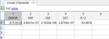
Not a good fit as R^2 value is less than 0.95 .

• Cubic Character

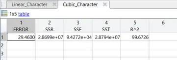
Good fit as R^2 value is greater than 0.95 .

Splitwise Method:

In order to reduce error, we'll be dividing the cp data into equal 8 groups. We'll be using the cubic relation as it has much better R^2 value, than the linear relation. Then we will calculate the coeff. and predicted values using the similar process for all of the 8 sets. After getting all the predicted cp values for 8 sets, we will combine them in one single array. and use it to compare it with the original data set.

• MATLAB CODE:

%Curve Fitting
%Splitwise

%Now we'll be divinding cp data into 8 sets

%set1
temp_01 = temp(1:400);
cp_01 = cp(1:400);
coeffs_01 = polyfit(temp_01, cp_01,3);
predicted_cp_01 = polyval(coeffs_01, temp_01);

%set2
temp_02 = temp(401:800);
cp_02 = cp(401:800);
coeffs_02 = polyfit(temp_02, cp_02,3);
predicted_cp_02 = polyval(coeffs_02, temp_02);

%set3
temp_03 = temp(801:1200);
cp_03 = cp(801:1200);
coeffs_03 = polyfit(temp_03, cp_03,3);
predicted_cp_03 = polyval(coeffs_03, temp_03);

%set4
temp_04=temp(1201:1600);
cp_04 = cp(1201:1600);
coeffs_04 = polyfit (temp_04, cp_04, 3);
predicted_cp_04 = polyval(coeffs_04, temp_04);

%set5
temp_05=temp(1601:2000);
cp_05 = cp(1601:2000);
coeffs_05 = polyfit(temp_05, cp_05,3);
predicted_cp_05 = polyval (coeffs_05, temp_05);

%set6
temp_06=temp(2001:2400);
cp_06 = cp(2001:2400);
coeffs_06 = polyfit(temp_06, cp_06,3);
predicted_cp_06 = polyval(coeffs_06, temp_06);

%set7
temp_07=temp(2401:2800);
cp_07 = cp(2401:2800);
coeffs_07 = polyfit(temp_07, cp_07,3);
predicted_cp_07 = polyval(coeffs_07, temp_07);

%set8
temp_08=temp(2801:3200);
cp_08 = cp(2801:3200);
coeffs_08 = polyfit(temp_08, cp_08, 3);
predicted_cp_08 = polyval(coeffs_08, temp_08);

predicted_cp=[predicted_cp_01; predicted_cp_02; predicted_cp_03; predicted_cp_04;
    predicted_cp_05; predicted_cp_06; predicted_cp_07; predicted_cp_08];

%Plotting
plot(temp, predicted_cp, 'linewidth', 3, 'color', 'y');
hold on
plot (temp, cp, 'linewidth', 1, 'color', 'r');
xlabel('Temperature [K]');
ylabel('Specific Heat Capacity [KJ/Kmol-K]');
legend ('split Curve', 'Original Data Set');
legend ('Location', 'northwest');

%Fitness Check
error=(cp-predicted_cp);
avg=mean(error.^2);
SSE=sum(avg);

SSR=sum((predicted_cp - mean(cp)).^2);

SST=SSR+SSE;

R_squared=SSR/SST;
R_squared_percentage=R_squared*100;

Splitwise_character=table(avg, SSR, SSE, SST, R_squared_percentage);
Splitwise_character.Properties.VariableNames={'ERROR', 'SSR', 'SSE', 'SST', 'R^2'};

OUTPUT:

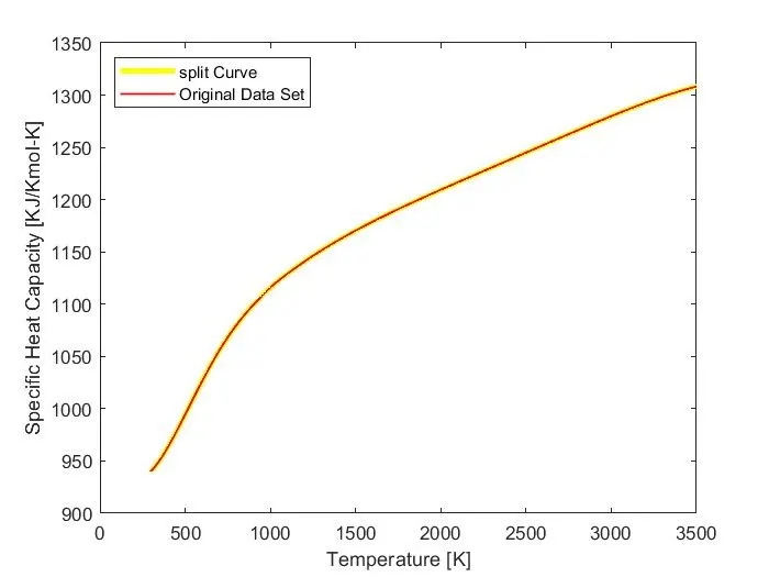
• Splitwise Character:

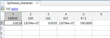
Thus, this is the best fit as the R^2 value is 1.

Q1. How to make a curve fit perfectly?

Ans. In order to make perfect fit, we must consider error estimates as well. Perfect fit means, the curve should fit the original curve without showing any errors (such as centering and scaling erros) in that perticular degree of polynomial.

Q2.How to get the best fit?

Ans. In order to get the best fit, it is important to reduce errors as much as possible. One of the ways to get a best fit is to use splitwise method. A perfect fit can always be a best fit, but a best fit can't always be a perfect fit. By increasing the degree of our polynomial, we might get best fit, but it can also be an overfit.

Q3.What could be done to improve the cubic fit?

Ans. We used splitwise method to improve our cubic fit. Than is one of the methods.