Week 3 - Solving second order ODEs
AIM:To write a program that solves the following ODE, which represents the equation of motion of a simple pendulum with damping.
In the above equation, g = gravity in m/s2, L = length of the pendulum in m, m = mass of the ball in kg, b=damping coefficient.
THEORY:
A damped oscillation means an oscillation that fades away with time. Examples include a swinging pendulum, a weight on a spring, and also a resistor - inductor - capacitor (RLC) circuit.
In the damped simple harmonic motion, the energy of the oscillator dissipates continuously. But for a small damping, the oscillations remain approximately periodic. The forces which dissipate the energy are generally frictional forces.
SOLVING 2nd ORDER ODE:
Here, we'll convert 2nd order ode into system of 1st order ode(s).
Let's say,
theta=theta_1 ..........(1)
dtheta1_dt=theta2 ..........(2)
then
d^2theta_dt^2=dtheta2_dt
thus, the eqn becomes,
dtheta2_dt=-(b/m)*theta2-(g/l)*sin(theta1) ...........(3)
Clubbing (2) & (3) in matrix form,
function [dtheta_dt]=ode_function(b,g,l,m,t, theta)
theta1=theta (1);
theta2=theta (2);
dtheta1_dt=theta2;
dtheta2_dt=-(b/m)*theta2-(g/l)*sin(theta1);
dtheta_dt=[dtheta1_dt;dtheta2_dt];
end
Matlab Code:
%Solving second order ODEs
clear all
close all
clc

%Setting fixed parameters
L=1; %metre
m=1; %kg
b=0.05; %Damping constant
g=9.81; %m/s2

%initial condition
theta_0=[0;3];

%solving ode
time=linspace(0,20,200);
[t,result]=ode45 (@(t, theta) ode_function(b,g,1,m,t,theta), time, theta_0);

%plotting
figure (1)
hold on
plot(t, result(:,1), 'color', 'r');
plot(t,result(:,2), 'color', 'b');
xlabel('Time')
ylabel('Displacemt/Velocity')
legend('Displacement', 'Velocity')
grid on

%creating animation
ct=1;

for i=1:length(t)
    x0=0;
    y0=0;
    x1=1* sin(result(i,1));
    y1=-1*cos(result(i,1));
    figure(2)
    plot([-2 2], [0 0], 'linewidth', 3, 'color', 'r');
    line ([x0 x1], [y0 y1], 'linewidth',4);
    axis ([-2 2 -2 2])
    hold on
    plot (x1, y1, 'o', 'markers', 20, 'markerfacecolor','g');
    hold off
    grid on
    pause (0.03);
    M(ct)=getframe(gcf);
    ct=ct+1;
end

movie (M)
videofile=VideoWriter('Second_order_ODE.avi', 'uncompressed avi');
open (videofile)
writeVideo(videofile,M)
close (videofile)

%ode function
function [dtheta_dt]=ode_function(b,g,l,m,t, theta)
theta1=theta (1);
theta2=theta (2);
dtheta1_dt=theta2;
dtheta2_dt=-(b/m)*theta2-(g/l)*sin(theta1);
dtheta_dt=[dtheta1_dt;dtheta2_dt];
end- Under %solving ode, we have used an built-in matlab function 'ode45', which is an built-in ode solver. Here we are solving for 't' and 'theta' and 'time' is the time span for which we are solving and 'theta_0' is the initial condition.
- The 'ode_function' returns 'dtheta_dt' matrix, which contains 2 rows (see equation 4 above). The 'ode45' function solves for t and theta and returns the values in 'results'. First column of results contain values of Theta or angular displacement, second column contains the angular velocity.
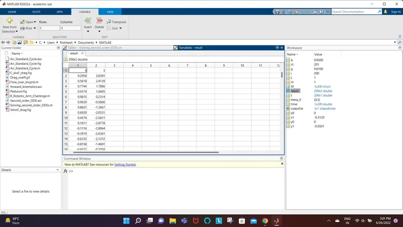
- Using the data in 'results', we plot the graph of displacement/velocity vs time.
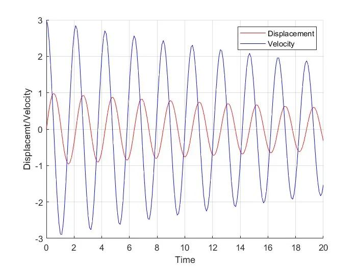
- From the graph, we can observe that the peak values of both, displacement and velocity decreases with time.
CREATING ANIMATION:
- To create an animation, we will save each figure in matrix 'M', and use the 'Movie' command to create a movie of those figures/frames by using the command 'getframe' and a counter variable 'ct'.
- To do so, we'll be using a for loop, where we'll be using the values of 1st column of results one by one to get the co-ordinates of the moving point, 'x1' & 'y1', which will also act as the center for the sphere which we'll be creating using 'marker' command.
- Once the for loop ends, in order to save the animation, we'll create a 'videofile' variable using the command 'VideoWriter', specifing the name of the file and it's format.
- The 'writeVideo' command writes the movie 'M' into the variable 'videofile', thus saving the animation.
LINK FOR THE ANIMATION: https://youtu.be/RIpBeFOkym4