Project 2 - Rankine cycle Simulator
AIM: To create a Rankine Cycle Simulator using MATLAB.
OBJECTIVES:
- The code should calculate the state points of the Rankine Cycle (any type of your choice) based on user inputs.
- Then, plot the corresponding T-s and h-s plots for the given set of inputs. Title and axes labels are a must, while legends could be used if necessary.
- Attach a report explaining the working of a rankine cycle simulator and also the research done by you.
THEORY:
The Rankine cycle is an idealized thermodynamic cycle describing the process by which certain heat engines, such as steam turbines or reciprocating steam engines, allow mechanical work to be extracted from a fluid as it moves between a heat source and heat sink. The Rankine cycle is named after William John Macquorn Rankine, a Scottish polymath professor at Glasgow University.
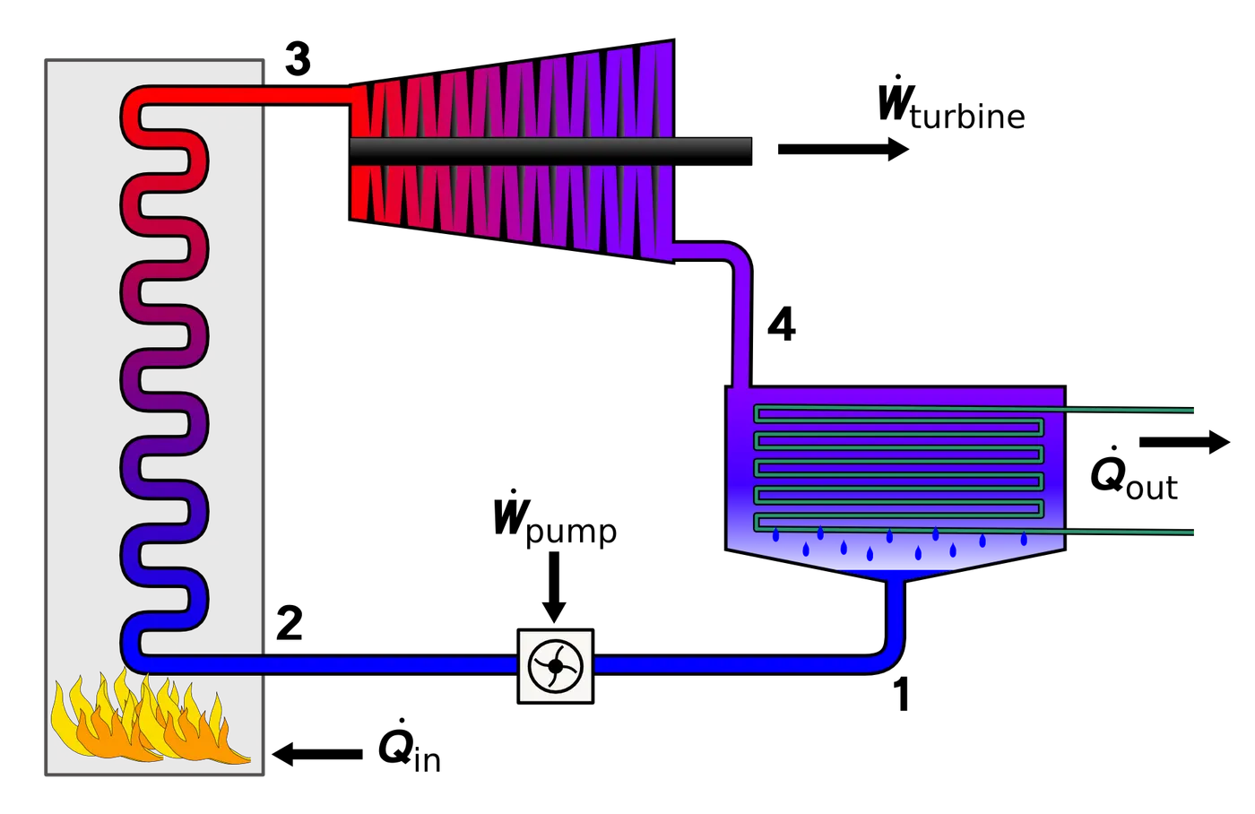
Physical layout of the Rankine cycle 1. Pump, 2. Boiler, 3. Turbine, 4. Condenser
The Rankine cycle makes practical use of the increase in pressure that occurs when a condensed fluid is forced to evaporate within a contained vessel. The cycle begins when a fluid, such as water, is compressed and put under high pressure. When the liquid is heated, the compressed fluid becomes a vapor that can be used to generate mechanical energy. When the heat is reduced, the vapor cools and condenses back to liquid form. The cycle then begins again.
A system that uses the Rankine cycle has four parts: a pump, a boiler, a turbine and a condenser. The pump's job is to deliver liquid to the boiler. The boiler's job is to heat the liquid and turn it to vapor. The vapor is then used to power a turbine. The turbine's job is to transform the energy created by the heated fluid into usable energy. The vaporized liquid is then cooled back to liquid state in the condenser. The pump pressurizes the liquid in the condenser and the cycle continues.
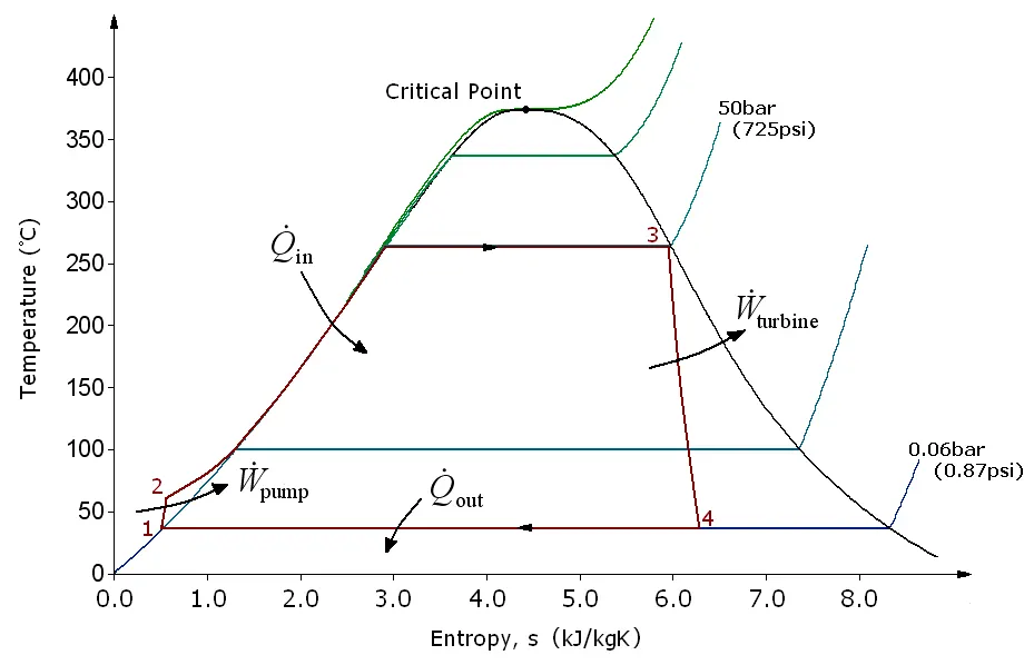
The four processes in the Rankine cycle are as follows:
- Process 1–2: The working fluid is pumped from low to high pressure. As the fluid is a liquid at this stage, the pump requires little input energy. Process 1-2 is isentropic compression.
- Process 2–3: The high-pressure liquid enters a boiler, where it is heated at constant pressure by an external heat source to become a dry saturated vapour. The input energy required can be easily calculated graphically, using an enthalpy–entropy chart (h–s chart, or Mollier diagram), or numerically, using steam tables or software. Process 2-3 is constant pressure heat addition in boiler.
- Process 3–4: The dry saturated vapour expands through a turbine, generating power. This decreases the temperature and pressure of the vapour, and some condensation may occur. The output in this process can be easily calculated using the chart or tables noted above. Process 3-4 is isentropic expansion.
- Process 4–1: The wet vapour then enters a condenser, where it is condensed at a constant pressure to become a saturated liquid. Process 4-1 is constant pressure heat rejection in condenser.
MATLAB CODE:
clear all
close all
clc

% Rankine Cycle Simulator

fprintf(' Rankine Cycle\n ')
fprintf('1-2 is Isentropic Expansion in Turbine\n')
fprintf(' 2-3 is constant pressure heat removal\n')
fprintf(' 3-4 is Isentropic Compression in Pump \n')
fprintf(' 4-1 Constant pressure Heat addition in Boiler\n')

% Entering the input data for calculation of state points
p1 = 30;        %Pressure at Turbine Inlet
T1 = 400;       %Temperature at Turbine Inlet
p2 = 0.05;      %Pressure at Condenser

% Taking data from Xsteam file for State point 1
h1 = XSteam('h_pT', p1, T1);        % Enthaply at pressure and Temp 1
s1 = XSteam('s_pT', p1, T1);        % Entropy at pressure and Temp 1

% Taking data from Xsteam file for State point 2
s2 = s1;                            % Because of Isentropic Expansion
sf2 = XSteam('sL_p', p2);           % Saturated liquid entropy at pressure 2
sg2 = XSteam('sV_p', p2);           % Saturated vapour entropy at pressure 2
x2 = (s2-sf2)/(sg2-sf2);            % Vapour Fraction at state point 2
hf2 = XSteam('hL_p', p2);           % Saturated liquid Enthalpy at pressure 2
hg2 = XSteam('hV_p', p2);           % Saturated vapour Enthalpy at pressure 2
h2 = hf2 + (x2*(hg2-hf2));          % Enthalpy at state point 2

% Taking data from Xsteam file for state point 3
p3 = p2;                            % Constant Pressure heat removal process
s3 = XSteam('sL_p', p3);            % Saturated liquid entropy at Pressure 3
h3 = XSteam('hL_p', p3);            % Saturated liquid Enthalpy at Pressure 3

% Taking data from Xsteam file for State point 4
s4 = s3;                            % Isentropic Compression process
p4 = p1;                            % Constant Pressure heat rejection

% Work done in Turbine for the rankine cycle
W_T = h1-h2;

% Work done required for pump
v3 = XSteam('vL_p',p3);             % Saturated Liquid Vapour at pressure 3
W_P = v3*(p4-p3)*100;               % Work done for pump
h4 = h3 - W_P;                      % Enthalpy at State point 4

% Net work done for Rankine Cycle
W_net = W_T - W_P;

% Heat Addition to System
Q_in = h1-h4;

% Heat Rejection from System
Q_out = h2-h3;

% Thermal Efficiency of Rankine Cycle
T_eff = (W_net/Q_in)*100;

%specific steam consumption  = (Mass flow rate / Net work done)
Sp_S = (3600/W_net);

% Calculation of Temperature at All state Point 2, 3 and 4
T3 = XSteam('Tsat_p',p3);           % Saturation Temperature at Pressure 3
T2 = T3;                            % Becuase of Constant Pressure Heat addition
Cp4 = XSteam('Cp_ps',p4,s4);        % Specific isobaric heat capacity
Cv4 = XSteam('Cv_ps',p4,s4);        % Specific isochoric heat capacity
k = Cp4/Cv4;
T4 = T3/((p3/p4)^((k-1)/k));        % Temperature at State point 4

% Calculation of Other constant for saturated liquid and Vapour
T6 = XSteam('Tsat_p', p1);          % Saturated Temperature at Pressure 1
s5 = XSteam('sL_p', p1);            % Saturated Liquid entropy at pressure 1
s6 = XSteam('sV_p', p1);            % Saturated Vapour entropy at Pressure 1
h5 = XSteam('hL_p', p1);            % Saturated Liquid Enthalpy at Pressure 1
h6 = XSteam('hV_p', p1);            % Saturated Vapour Enthalpy at pressure 1
T5 = T6;

%Plotting for Saturation Line
T = linspace(1,560,1000);
for i = 1:length(T)
    sf(i) = XSteam('sL_T' ,T(i));   % Saturated Liquid Entropy
    sg(i) = XSteam('sV_T' ,T(i));   % Saturated Vapour Entropy
    hf(i) = XSteam('hL_T' ,T(i));   % Saturated Liquid Enthalpy
    hg(i) = XSteam('hV_T' ,T(i));   % Saturated Vapour Enthalpy

end

% Plotting T-S Diagram for Rankine Cycle
figure(1)
hold on
plot(sf,T,'color','b','linewidth',2)
plot(sg,T,'color','b','linewidth',2)
plot([s1 s2],[T1 T2], 'color', 'r', 'linewidth',3)
plot([s2 s3],[T2 T3], 'color', 'r', 'linewidth',3)
plot([s3 s4],[T3 T4], 'color', 'r', 'linewidth',3)
plot([s4 s5],[T4 T5], 'color', 'r', 'linewidth',3)
plot([s5 s6],[T5 T6], 'color', 'r', 'linewidth',3)
s_1 = linspace(s6,s1,1000);
for j = 1:length(s_1)
    Tc(j) = XSteam('T_ps',p1,s_1(j));
end
plot(s_1,Tc,'color','r','linewidth',3)
text(s1+0.1, T1, '1')
text(s2+0.1, T2, '2')
text(s3, T3-20, '3')
text(s4, T4+20, '4')
title('Temperature Vs Entropy')
xlabel('Entropy (Kj/kg-k)')
ylabel('Temeperature (Deg. Celcius)')
legend('Saturation Curve')

% Plotting H-S Diagram for Rankine Cycle
figure(2)
hold on
plot(sf,hf,'color','b','linewidth',2)
plot(sg,hg,'color','b','linewidth',2)
plot([s1 s2],[h1 h2],'color','r','linewidth',3)
plot([s2 s3],[h2 h3],'color','r','linewidth',3)
plot([s3 s4],[h3 h4],'color','r','linewidth',3)
hc = linspace(h4,h5,100);
for k = 1:length(hc)
    s_c(k) = XSteam('s_ph',p1,hc(k));
end
plot(s_c,hc,'color','r','linewidth',3)
plot([s5 s6],[h5 h6],'color','r','linewidth',3)
for l = 1:length(s_1)
    h_c(l) = XSteam('h_ps',p1,s_1(l));
end
plot(s_1,h_c,'color','r','linewidth',3)
text(s1+0.1,h1,'1')
text(s2+0.1,h2,'2')
text(s3,h3-100,'3')
text(s4,h4+200,'4')
title('Enthalpy Vs Entropy')
xlabel('Entropy (Kj/kg-k)')
ylabel('Enthalpy (KJ/Kg)')
legend('Saturation Curve')

% Displaying Results in Command window
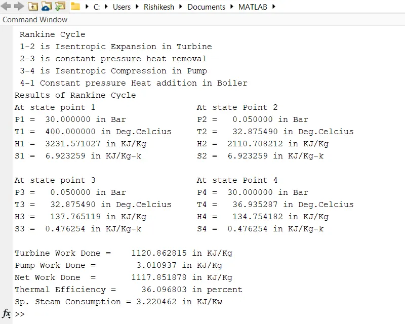
disp('Results of Rankine Cycle')
fprintf('At state point 1\t\t\t\t\t')
fprintf('At state Point 2\n')
fprintf('P1 = %10f in Bar\t\t\t\t',p1);
fprintf('P2 = %10f in Bar\n',p2);
fprintf('T1 = %11f in Deg.Celcius\t\t',T1);
fprintf('T2 = %11f in Deg.Celcius\n',T2);
fprintf('H1 = %12f in KJ/Kg\t\t\t',h1);
fprintf('H2 = %12f in KJ/Kg\n',h2);
fprintf('S1 = %9f in KJ/Kg-k\t\t\t',s1);
fprintf('S2 = %9f in KJ/Kg-k\n',s2);
fprintf('\n')
fprintf('At state point 3\t\t\t\t\t')
fprintf('At state Point 4\n')
fprintf('P3 = %10f in Bar\t\t\t\t',p3);
fprintf('P4 = %10f in Bar\n',p4);
fprintf('T3 = %11f in Deg.Celcius\t\t',T3);
fprintf('T4 = %11f in Deg.Celcius\n',T4);
fprintf('H3 = %12f in KJ/Kg\t\t\t',h3);
fprintf('H4 = %12f in KJ/Kg\n',h4);
fprintf('S3 = %9f in KJ/Kg-k\t\t\t',s3);
fprintf('S4 = %9f in KJ/Kg-k\n',s4);
fprintf('\n')
fprintf('Turbine Work Done = %14f in KJ/Kg\n',W_T)
fprintf('Pump Work Done = %15f in KJ/Kg\n',W_P)
fprintf('Net Work Done  = %17f in KJ/Kg\n',W_net)
fprintf('Thermal Efficiency = %13f in percent\n',T_eff)
fprintf('Sp. Steam Consumption = %f in KJ/Kw\n',Sp_S)
EXPLANATION:
- First we input the initial conditions required for the cycle to operate (eg. turbine inlet pressure etc).
- Then using the XSteam functions file, we get the value of enthalpy and entropy at state point 1.
- As 1-2 process is an isentropic compression process, the entropy at point 1 is equal to point 2. The term ‘(s_pT, p1, T1)’ refers to entropy at pressure and temperature point 1.
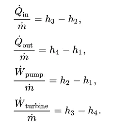
- Similarly, other points are taken from XSteam function file which are necessary to calculate other parameters. After that work done in turbine and pump are calculated for further getting the net work done Rankine cycle. The equations used are:

5.After calculating the net work done the efficiency of the Rankine cycle is calculated along with specific steam consumption which is steam consumed by a locomotive cylinders per unit of output of work done.
6.Then temperature at each point of cycle is calculated using input taken from start of the program and data taken from XSteam file. For given temperature range from lower to higher entropy points are calculated to create the T-S plot. Similarly, another for loop is used to create the saturation curve in each plot.
7.Then plotting is done respectively for T-s and H-s graph in Rankine cycle and each state point value has been put in command window.
OUTPUTS:
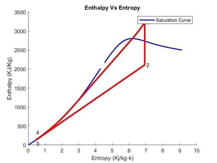
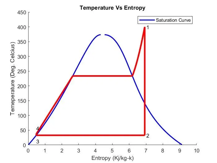
COMMAND WINDOW:
REFERENCES:
https://en.wikipedia.org/wiki/Rankine_cycle
https://www.techtarget.com/whatis/definition/Rankine-le#:~:text=The%20Rankine%20cycle%2C%20also%20called,the%20thermodynamic%20properties%20of%20steam.