Week - 4 - Crash Box Simulation
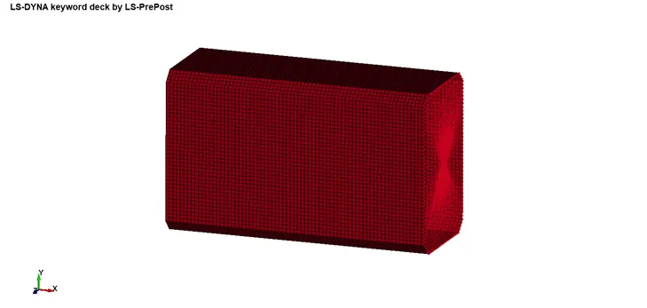
Crash test of rectangular box tube
Introduction:
In this simulation example, the crash box is impacted with some initial velocity on the rigid wall in order to observe the energy absorbing behavior of the box. In order to verify those behavior, cross sectional force is monitored along with the total energy of the tube with time. Each data is entered in g, mm, ms unit system.
Modeling and Keywords:
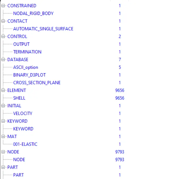
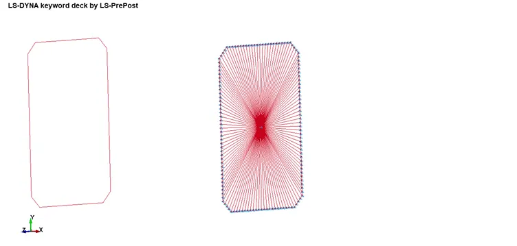
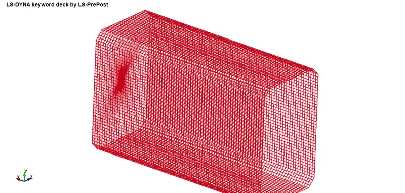
Constrained nodal rigid body is shown below. It is a set of node of CNRB type which is required to provide equal velocity to the each node at the end of tube.
Automatic single surface contact is create to prevent unrealistic penetration of the body during collision or distortion or contact due to large displacements.
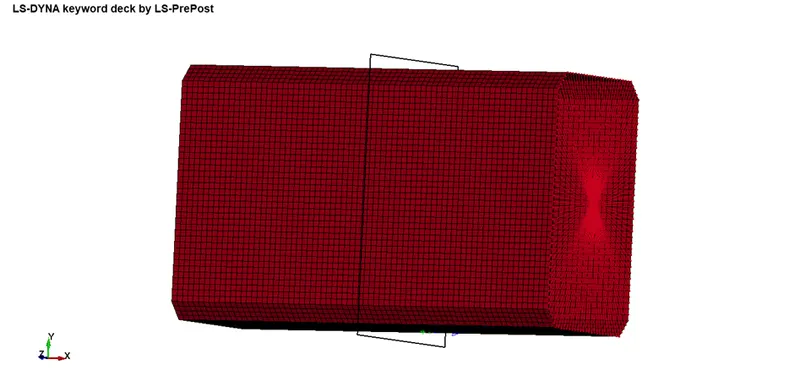
Cross-section plane is created at the middle of the tube so that we can evaluate the force generated on the plane during each time.
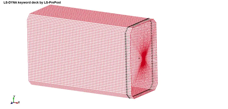
Initial velocity is provided to the CNRB node set of 50 km/h and also to the whole body excluding CNRB to check the difference in the results of the different method of assigning the velocity:
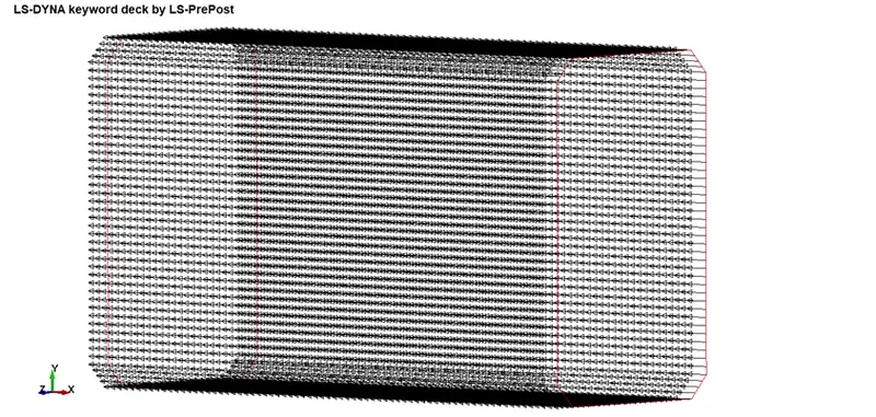
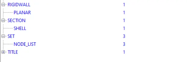
Rigid wall is created as shown below perpendicular to the length of the tube.
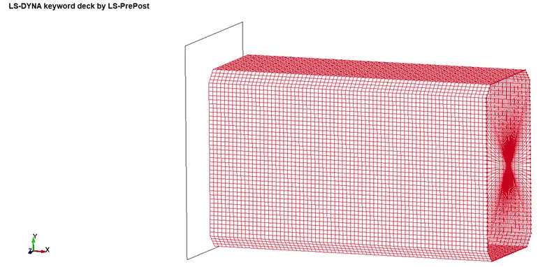
Analysis:
In this analysis, the velocity is assigned over the whole body instead of only at the CNRB node set because the simulation is more stable in former method.
Total energy of the system:
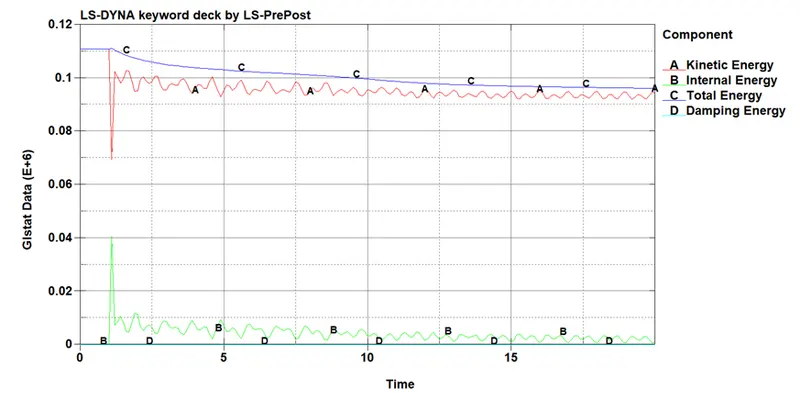
From above plot, it is clear that the energy of the system was conserved before hitting the rigid wall. After hitting the rigid wall, some of the energy is lost due to the increase damping energy. The percentage of loss of damping energy is below 10% hence it is acceptable for the simulation verification. (Velocity is subjected to the whole body node set in this case).
Acceleration of a middle node:
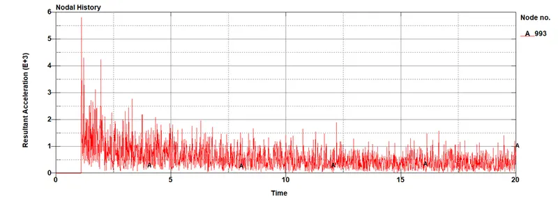
The resultant acceleration of the body is almost 0 which is true for the initial constant velocity. After impact of the tube with the rigid wall the tube acceleration kept fluctuating over time with positive mean acceleration.
Cross-sectional force at the middle:
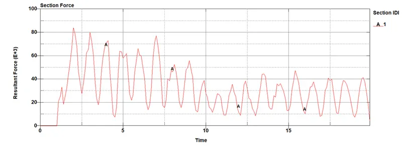
The sectional force acting on the tube at the middle is also zero at the start then after the sectional force has exceeded the value 80 GPa which is way beyond the yield strength of the steel. As the simulation is linear in nature hence no non linearity is considered in this case. The sectional force in the middle decreased after some time after bouncing back. (Filter of 60 Hz and 4 point average is taken in above graph)
Comparison between 1.5 and 1.2 mm thick tube:
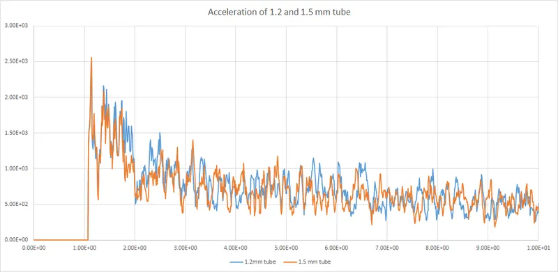
The thickness of the tube has very little effect on the acceleration. As we can see the maximum and average range of fluctuation of the acceleration is almost similar in both the cases. The data over here is shown only for the 10ms because it is same for other time too. (Filter of 60 Hz and 4 points average is taken in above graph).
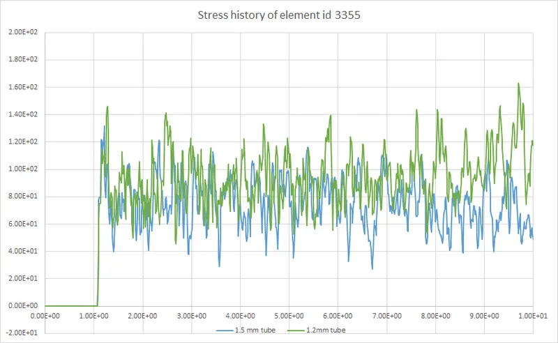
From above plot we can imply that the stress in the tube with less thickness is higher than the tube with higher thickness which is logical. This can also be taken as a way of validating the simulation. (Filter of 60 Hz and 4 points average is taken in above graph).
Learning outcomes:
- The thickness effect over the stress distribution
- Variation in result due to different way of assigning the initial velocity
Conclusion:
The different method of assigning the velocity can give different output so one need to be aware of the method appropriate for their problems and the stress concentration will decrease with increasing thickness of the object due to increase area of the objects.