Week - 4 - crash box simulation

Skill-lync assignment 4

Aim: The objective of this assignment is to pre-process the given input file, simulate a crash test and compile results of the same.

Case setup: The given input file is a mesh of a simple rectangular crash tube and is shown below. The component is to worked on while using the kg, mm, ms units.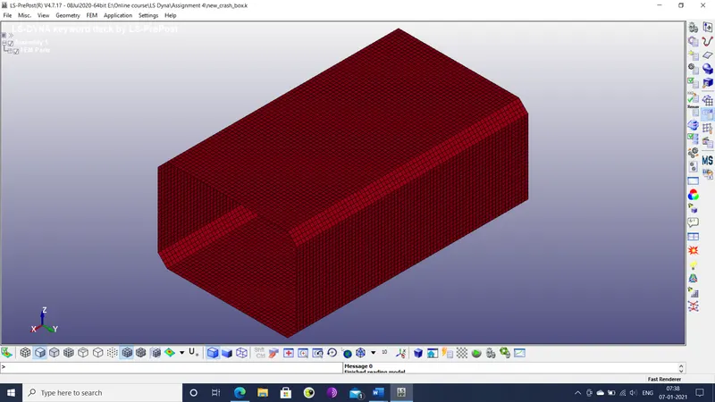

Figure 1: Crash tube

Boundary conditions: The crash tube is to have the following boundary conditions: -

1. Material: Steel (Elastic behavior)
2. Thickness: 1.2 mm (1^st iteration), 1.5 mm (2^nd iteration)
3. Initial velocity: 50 kmph or 13.8889 mm/ms

Output files: The following plots & output files are to be derived through post-processing: -

1. D3plot, glstat, sleout and rcforce output files.
2. Cross-sectional force in longitudinal direction.
3. Acceleration of a node in the middle of the crash tube.
4. Longitudinal stress and strain
5. Total, internal, kinetic, hourglass and sliding energies.

Procedure: The given input file is pre-processed and post-processed through the following sequence of steps: -

1. The input file is imported into the LS PrePost workspace.
2. The part is assigned a section with a thickness of 1.2 mm and an element formulation type 16 (Fully integrated shell element) through the SECTION_SHELL keyword. This section is then assigned to the crash tube part.
3. Steel with isotropic elastic failure behavior is assigned to the part via the MAT>24_PIECEWISE_LINEAR_PLASTICITY keyword. Referring to literature, the following properties are assigned to the material.

• Density: 7.8 X 10-6 kg/mm³
• Young’s modulus: 210 kg/(mm*ms²)
• Poisson’s ratio: 0.33
• Yield strength: 0.4 kg/(mm*ms²)
• Tangent modulus: 0.25 kg/(mm*ms²)
• Plastic failure strain: 0.14

A stress-strain curve is also defined for the material, as shown below.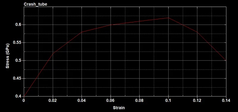

Figure 2: Stress-strain curve

4. A node set is created for the nodes in the crash tube via the create entity tool. The SET_NODE_LIST keyword is used for this purpose.
5. A rigid wall is created at the x-coordinate of 256 mm with a friction coefficient of 0.1. The node set defined earlier is set as the slave nodes of this rigid wall.
6. Self-contact is established within the crash tube via the CONTACT>AUTOMATIC_SINGLE_SURFACE keyword. The master set node ID is set as 0, signifying self-contact. The slave segment type (SSTYP) is set to 3 (part ID).
7. An initial velocity of 13.8889 mm/ms is applied to the node set defined for the crash tube via the INITIAL>VELOCITY keyword.
8. The CONTROL>CONTACT keyword is edited so that initial penetrations (ISLCHK: 2) and thickness changes (THKCHG: 1) are considered.
9. The CONTROL>HOURGLASS and CONTROL>SHELL keywords are added to the file.
10. The CONTROL>TERMINATION keyword is edited so that minimum time step (DTMIN) is 0.0005 ms and run time (ENDTIM) is 1 ms.
11. The DATABASE>ASCII_option keyword is edited to include glstat, rcforc and sleout files as output. In addition, minimum time interval between plot points (DT) is set as 0.01 ms and binary output is set as 3 (output in ASCII file and in binary file).
12. In order to measure cross-sectional force, a node set and a shell set are defined for the crash tube, as shown below.

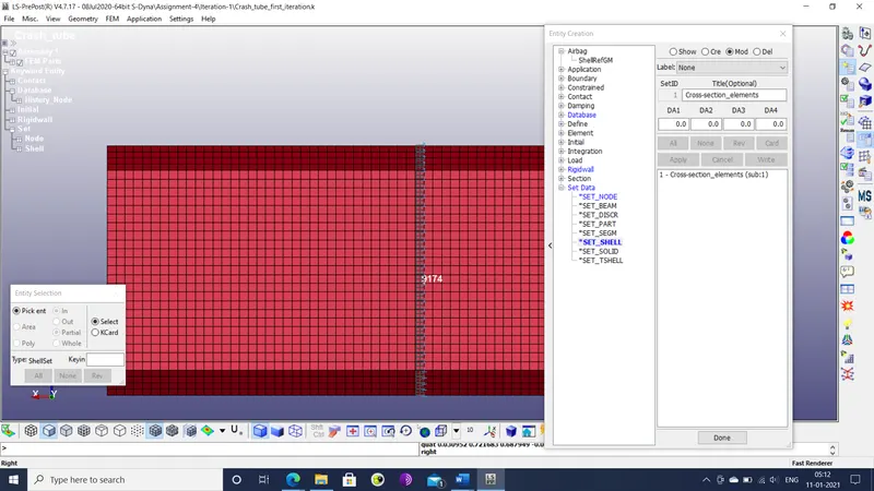
Figure 3: Shell element set for cross-section

13. The DATABASE>CROSS_SECTION_SET keyword is then edited to create a cross-sectional plane that passes through the node set defined. Also, the DATABASE>ASCII_option is edited so that resultant force is output into a secforc file.
14. The model checker is run to check the component for any errors in the keywords.
15. The keyword file is then saved and then run using the LS-Run software.
16. The resultant binary plot is imported into the LS-PrePost workspace.
17. The secforc file is loaded from the ASCII output and the resultant force history on the specified cross-section is plotted.
18. A node is selected in the middle of the tube and its acceleration history is plotted.
19. The maximum directional stresses and strains are plotted.
20. The total, internal, kinetic, sliding and hourglass energies are plotted from the glstat file.
21. A copy of the keyword file is modified so that shell thickness is 1.5 mm and then saved as a separate file.
22. Steps 16-20 are repeated for the second file.

Results: The various plots and observations are listed below.

1. The plot of the cross-sectional forces for the two iterations are shown below.

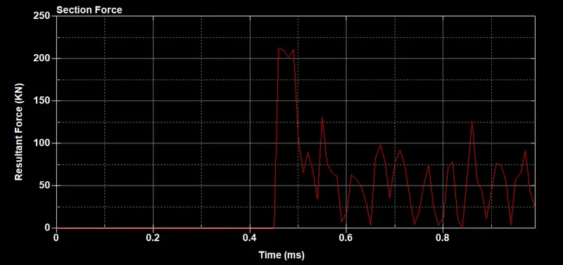
Figure 4: Cross-sectional force in 1.2 mm iteration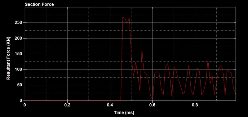

Figure 5: Cross-sectional force in 1.5 mm iteration

The plots are mostly similar, both showing a massive spike in resultant force during the moment of impact, followed by a persistent fluctuation in force indicating vibration within the crash tube. In the second iteration with shell thickness of 1.5 mm, the initial force spike is higher. This can be attributed to the greater mass of the second iteration due to the greater thickness.

2. The energy histories are plotted for both iterations below.

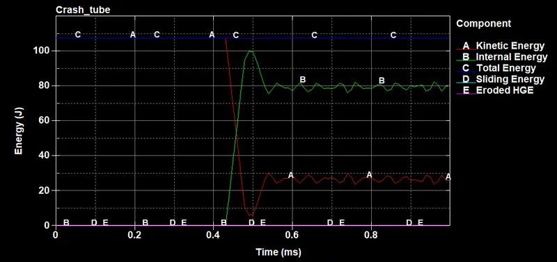
Figure 6: Energy plot in 1.2 mm iteration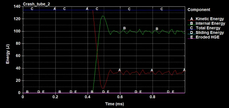

Figure 7: Energy plot in 1.5 mm iteration

They show similar plots which indicates consistent material behavior. Sliding and hourglass energy are practically non-existent, which confirms adequate element formulation and hourglass energy control. As a result, the overall plot matches the one that is to be expected from a real setup. The total energy is mostly constant. The drop in kinetic energy is mirrored by the rise in internal energy. This is followed by oscillations in both, indicating vibrations generated in the tube. As with the cross-sectional force, the overall energies are greater in the second iteration due to the same reason of greater mass.

3. The acceleration in the middle of the crash tube for both iterations are plotted below.

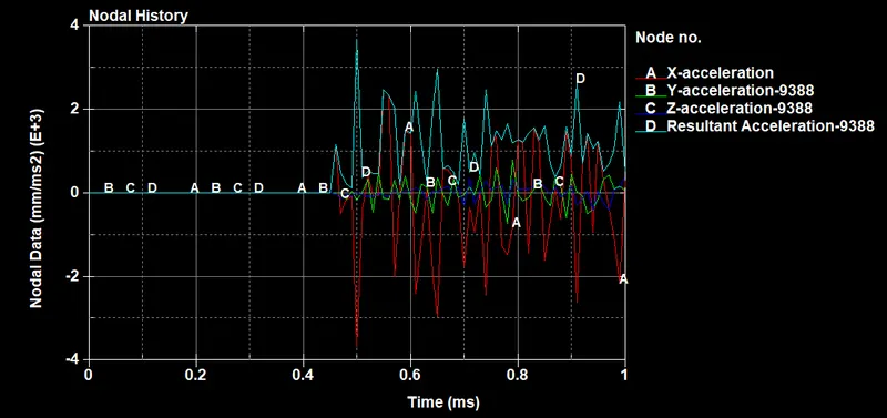
Figure 8: Acceleration plot for 1.2 mm iteration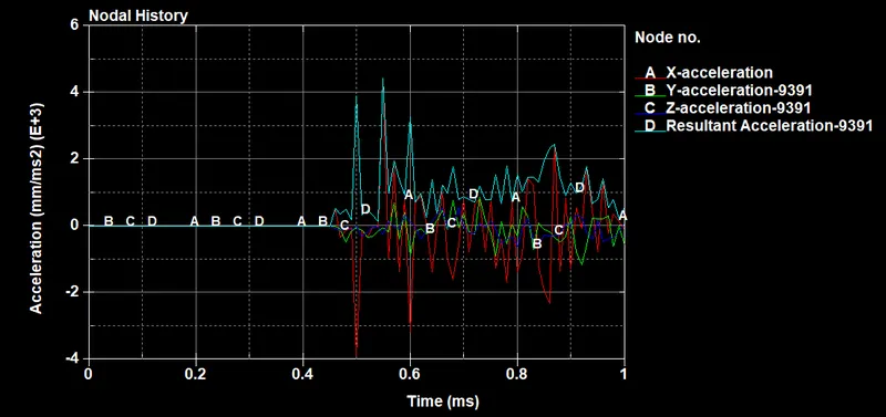

Figure 9: Acceleration plot for 1.5 mm iteration

The acceleration plots are not particularly consistent for both iterations. There is a small amount of accelerations in the y and z directions (along cross-section). However, the majority of the acceleration is in the x direction (lengthwise). It shows a large negative spike at the moment of impact, followed by persistent oscillations. The initial spike is roughly the same for both iterations, showing that the increased mass in the second iteration is not enough to influence deceleration. However, in the second iteration, the magnitude of oscillations was reduced due to the greater mass. Before the impact however, in both cases, there was a small positive acceleration, which might point to inaccuracies in the formulation of the rigid wall interface.

4. The maximum directional stresses for both iterations are shown below.

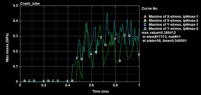Figure 10: Longitudinal (x direction) and transverse (y direction) stresses in 1.2 mm iteration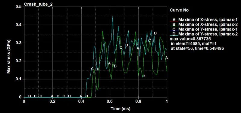

Figure 11: Longitudinal (x direction) and transverse (y direction) stresses in 1.5 mm iteration

They show cyclic variation in maximum stress in both the lateral and transverse directions. It also shows that maximum stress starts developing in the transverse direction (y). This might seem counter-intuitive, but this maximum stress plot only considers tension (positive maximum) and not the actual magnitude of the stress. While stress generated is most significant in the x-direction, this stress is compressive (negative) in nature. Ultimately, shell thickness does not seem to have any noticeable influence on these stresses.

5. The maximum directional strains for both iterations are shown below.

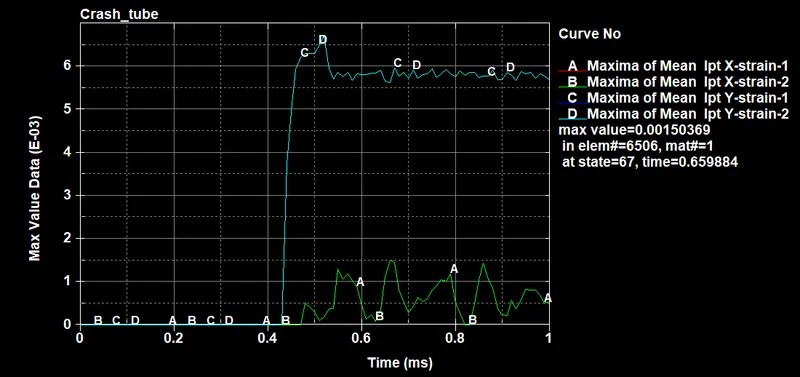Figure 12: Longitudinal (x-direction) and transverse (y-direction) strains in 1.2 mm iteration

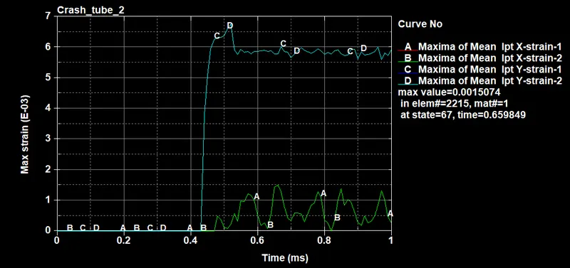Figure 13: Longitudinal (x-direction) and transverse (y-direction) strains in 1.5 mm iteration

They show that the magnitude of permanent (plastic) strain is very small, i.e. the tube does not undergo any significant deformation. The little plastic deformation that is observed is almost entirely in the longitudinal direction. The plots also show the persistent oscillations after the moment of impact. The shell thickness has no effect on any of the strains, as seem in the plots.

Conclusion: The given component has been successfully worked on in the LS-Dyna workspace and post-processed to analyze its behavior. The two iterations with different shell thicknesses were compared to see its influence on component performance.