Week - 4 - Crash Box Simulation
Title: Crash Analysis of a Crash Box using LS Dyna
Objective: To setup the simulation of a crash test of the crash box in LS Dyna with different shell thickness and get the deliverables.
Deliverables:
a. Input and Output files (.k, d3plot, glstat, nout, etc)
b. Cross section force generated at the half length of the crash box
c. Stress and Strain along the length of the box
d. Energy and acceleration plots for 1.2 and 1.5 mm shell thickness
Abstract:
Crash box is high energy absorbing device, the strcture of the box is such that in operation when the crash occurs, the loads result into the high deformation of the box and correspondingly less impact on the other components. A general crash box in automotive has a complicated design, in this example a general example of box is considered.
Following are the specifications of the simulation
Planar Rigid wall is used for the crash.
Linear Material (MAT 01 ) and Non Linear (MAT 98) with steel properties
Initial Velocity is 50kmph
Thickness of the box is 1.2 mm and 1.5 mm
Unit system followed is gm-mm-ms
Procedure:
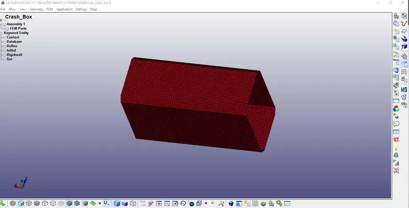
Importing the mesh file. The mesh file of the crash box is provided. The file is opened in LS - PrePost in order to setup the analysis.
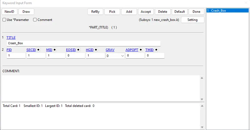
The imported mesh is given name using the Part Keyword as Crash Box. The next important thing to enter is the Shell Section property and the material details. Following figures show the Material and Section keyword cards used for the crash box.
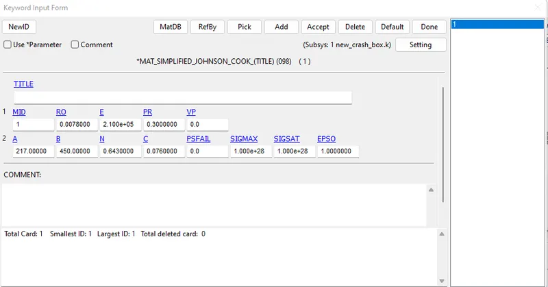
Material
The material used is Elastic for linear analysis and MAT98 (Simplified Johnson Cook) for non linear.
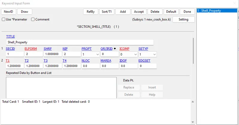
Section Property
In this analysis the crash box has two different thicknesses, 1.2 mm and 1.5 mm
The section id (SECID) and the material id (MATID) are entered in the Part card to define it to the Crash Box component.
Rigid Wall:
The next important component of the analysis is the Rigid wall. In this example the required type of rigid wall is planar. It is created using the entity creation option. The Rigid wall is placed at shorter distance from the end of the crash box, so that the required termination time is less. The friction is kept to 0 no friction is considered.
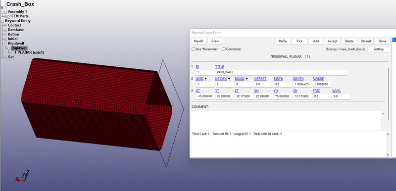
The slave nodes are defined using the Node Set, all the nodes are selected as the slave nodes.
Initial Velocity:
The crash box has the initial veolcity of 50kmph as the unit system used in the analysis is gm-mm-ms. It is converted into mm/ms, the value appears to be 13.88 mm/ms. In order to apply the initial velocity, the create entity option is used.
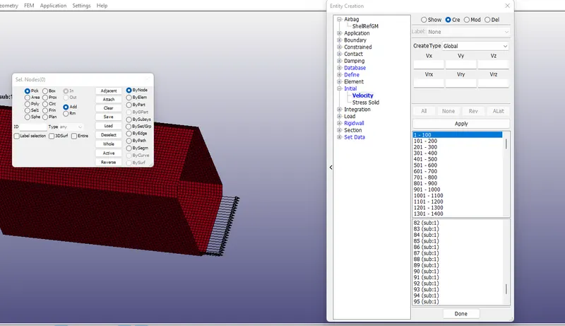
All the nodes are selected to apply the initial velocity. The value is entered for the Vx component as the component is aligned to X direction of global coordinate axes.
Contact:
It is unkonwn whether the crash buckles and comes in contact of itself. So Automatic Single Surface is used to apply the self contact. The slave component of the card is selected as the entire part, there is no need to add the master component. Using the part as the option of selection the part id is selected.
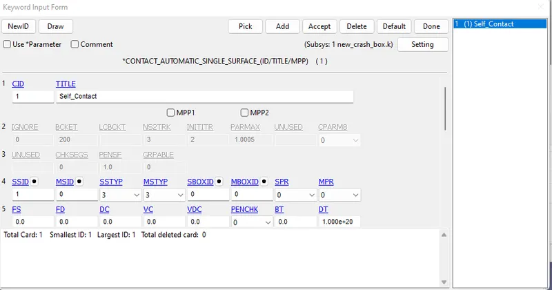
Hourglass:
In order to avoid the zero energy modes i.e Hourglass in the elements, the Hourglass keyword is used with the IHQ value as 2 and other default values.
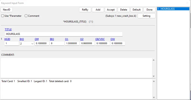
The Hourglass ID is selected in the part card of the part.
Output Requests:
Section Forces:
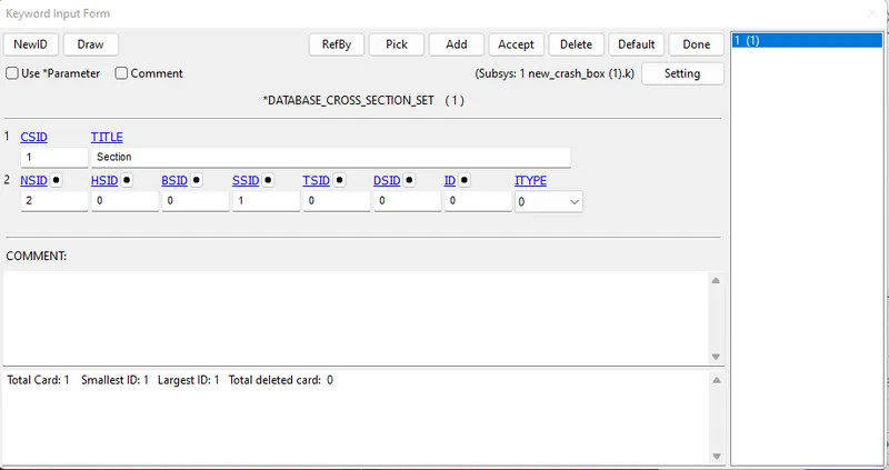
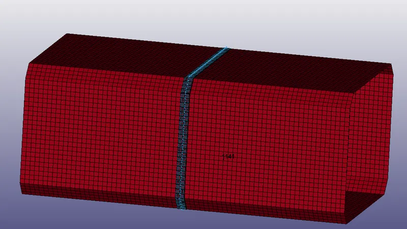
The sectional forces at the half of the length of the crash box are required. The section is created first using the create entity option. The Node and Shell set are created initially and are referred in the Cross section keyword card.
ASCII Output Requests:
Following output are requested,
a. ELOUT - Element Output Data
b. GLSTAT - Global Statistics
c. MATSUM - Material Energies
d. NODOUT - Nodal Outputs
e. RCFORC - Resultant Interface Forces
f. RWFORCE - Rigid Wall Force
h. SECFORC - Sectional Force
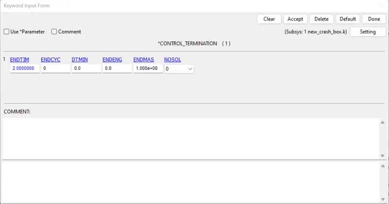
The output are requested for dt value as 0.01
Database Binary 3D Plot is requested with DT value as 0.01 and the total time for simulation 2 ms
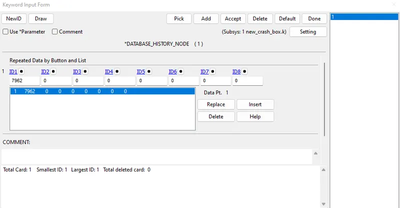
In order to get the nodal data, HISTORY_NODE keyword card is necessary to be used in the analysis.
Results:
a. Visual Animation of the Crash
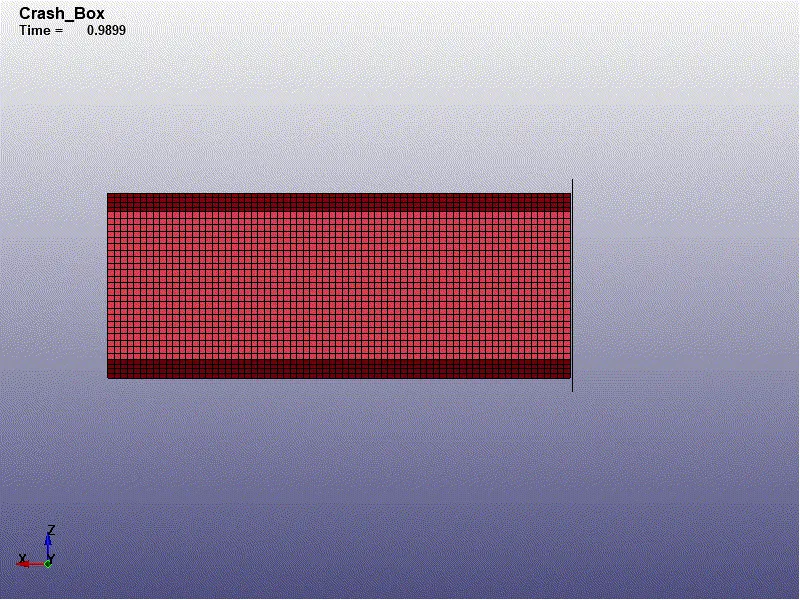
Stress Contour for Shell Thickness 1.2 mm
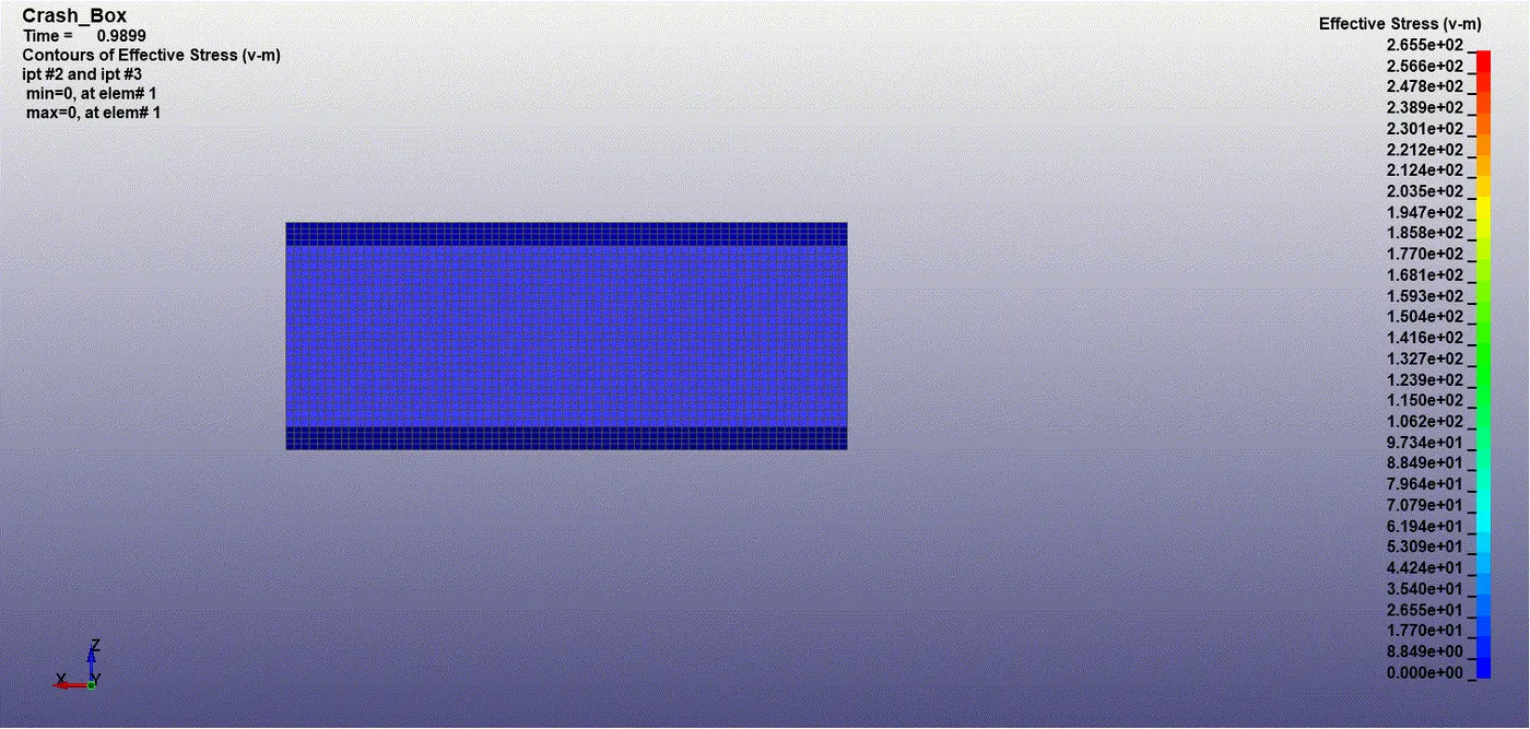
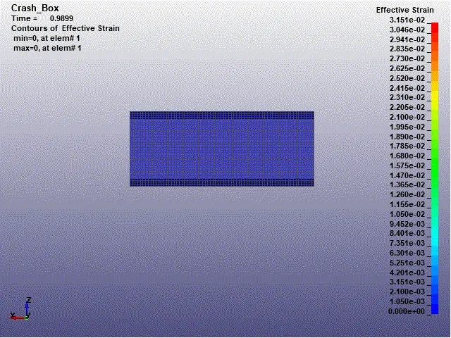
The stress at the point of contact is higher as it touches the rigid wall. The Von Misses stress surpass the yield stress value as it can be seen and hence the plastic strain will occur. If the plastic strain with Johnson Cook model is seen the value of plastic strain can be obtained.
Stress Strain Plot
Following Plot is for a random element in the box, the material for this model is Johnson Cook Model
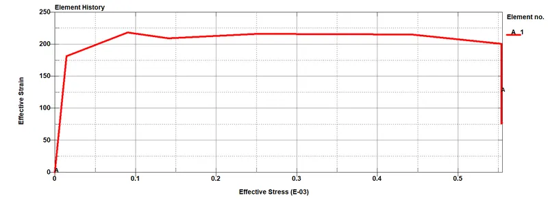
Maximum value of stress for this element is around 219 MPa and the plastic strain is around 0.05 %
Stress values for both the models
| Model | X Stress | Y Stress | Z Stress | X Strain | Y Strain | Z Strain |
| 1.2 mm | 243 | 141 | 147 | 0.00118 | 0.00127 | 0.00127 |
| 1.5 mm | 237 | 138 | 134 | 0.00126 | 0.00126 | 0.00123 |
Global Energy Plots:
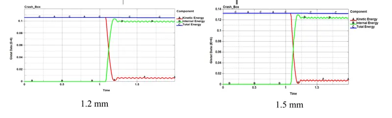
Above are the energy plots for 1.2 and 1.5 mm thickness model. It is clear that the energy conservation is obtained, the kinetic energy of the model is converted into the internal energy and for the model with 1.5 mm thickness the kinetic energy is higher than that of 1.2 mm, this is due to the mass of the second model being higher resulting into the higher kinetic energy. Also as the hourglass card was used and hence the hourglass is zero for the enitre duration of the analysis.
Acceleration Plot
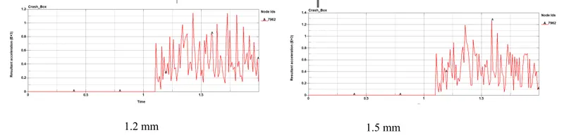
The plots above are the acceleration plots for the node at the centre of the crash box. No major varaition is seen in the curves as there is not a large difference in the physics of the problem, the velocity is same, the contact region is same.
Velocity Plot:
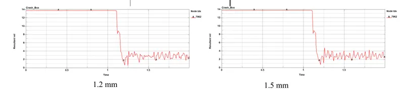
The velocity plot is shown the velocity of 13.8 is seen until the crash box contacts the rigid wall. Once the crash box impacts the rigid wall after impact it rebounds as seen in the animation.
Sectional Force:
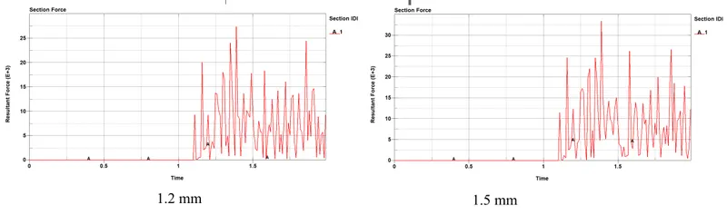
The sectional forces are plotted above for both the models. The forces are higher for 1.5mm model as the model posses higher Kinetic Energy compared to the 1.2mm model. Hence the reaction is higher and eventually higher forces are recorded.
Conclusion:
The setup for the crash box analysis was done in LS Dyna with two different shell thickness and the material.
The results for both the models are compared and the objectives were achieved.