Week - 4 - Crash Box Simulation
CRASH BOX SIMULATION
AIM: To create a complete simulation file for-crash analysis of a crash box having two
different thickness of 1.2 mm and 1.5 mm from the given FE model of the crash box and
produce the following deliverables.
Input. k file and output files (D3PLOT, GLSTAT, SLEOUT, RCFORC) Animation of the final simulation
The cross-sectional force generated in the middle of the crash box (along its length)
Acceleration plot of a node in the middle of the crash box (along its length)
Maximum directional stress and strain along the length of the crash box (X strain, Y
strain etc.)
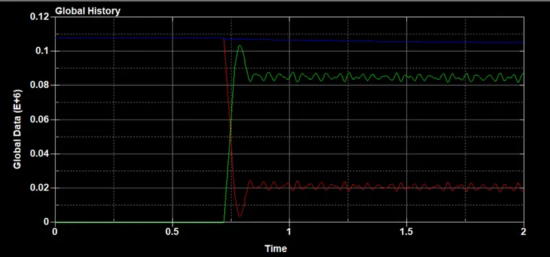
Plot of all energies (total, internal, kinetic, hourglass, sliding)
Compare the accelerations and stress/strain plots of 1.2/1.5mm crash boxes.
INTRODUCTION:
A crash box is a highly energy-absorbing structure that crashes on the application of loads and reduces the impact on other components nearby. A full-edged crash box is a highly sophisticated design but, in this case, a rectangular channel structure is considered as most simple crash box.
Following are the different assumptions and information required:
The crash box should crash into a rigid wall created using the *RIGIDWALL_ keyword.
The material for the crash box is steel.
The simulation should satisfy either of the two situations - (1) It crashes on the rigid wall and debounces completely or (2) it buckles and folds in the axial direction so as to come in self-contact.
Once the simulation is completed results are collected and another simulation is executed by increasing the thickness of the crash box from 1.2 mm to 1.5 mm.
PROCEDURE:
The given LS-Dyna keyword file is opened in LS-PrePost using the option.
File>Open>LS-Dyna Keyword File as shown.
Section properties:
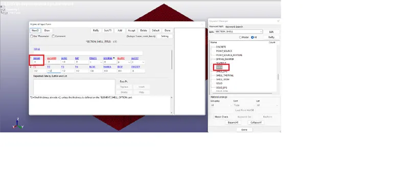
Keyword manager>SECTION>SHELL.
The section properties of the crash box are assigned as shell elements with 1.2 mm thickness
and ELFORM=2, Belytschko-Tsay element formulation.
Material properties:
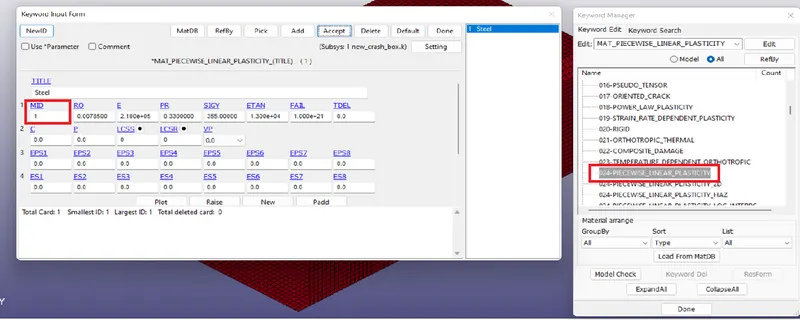
The crash box is assigned with steel material with the following parameters as shown in table.
Keyword manager>MAT>024-PIECEWISE LINEAR PLASTICITY.
MAT24 (Piecewise linear plasticity) material card is used to assign the steel material
properties to the crash box. The MAT24 represents Piecewise linear isotropic plasticity.
With this material model, it is possible to consider the effect of the strain rate.
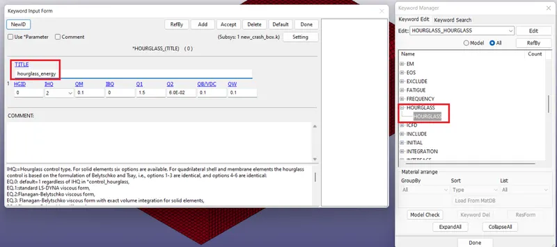
Viscous hourglass control is recommended for problems deforming with high velocities
i.e, Hourglass control type=IHQ=2, Flanagan-Belytschko viscous form.
Steel material properties Value
Mass Density [gm/mm] 7.85e-3
Young’s Modulus [MPa] 210e3
Poisson's ratio of 0.3
Yield stress [MPa] 355
Tangent modulus [MPa] 1.3e3
Keyword manager> HOURGLASS.
To avoid Hourglass energy generation, we will create an *HOURGLASS card with IHQ
value as 2 and the rest as default. Now assign this Hourglass card to the Crash_box
part. Viscous hourglass control is recommended for problems deforming with high.
Part definition:
Keyword manager>PART
The section, material, and hourglass ID are assigned to the part card respectively as shown.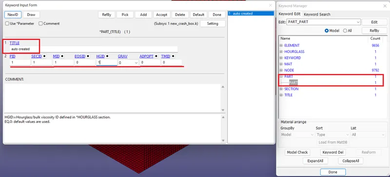
BOUNDARY CONDITIONS:
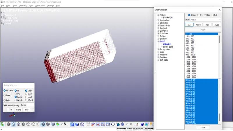
Initial Velocity:
Create Entity>Initial>Velocity>cre
The crash box is assigned with an initial velocity of V= -13.88 mm/ms is applied along +ve x
direction to crash against the rigid wall.
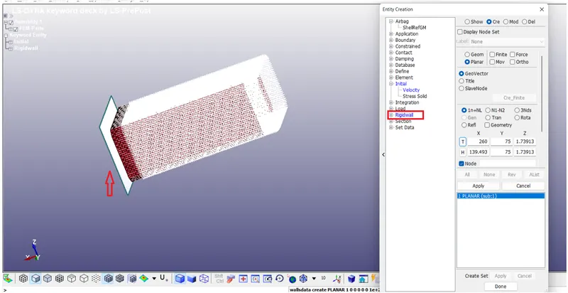
Rigid wall:
Create Entity>Rigidwall>cre>Planar>1n+NL
The rigid wall is created at a distance of 10mm away from the crash box.
CONTACT CONDITION:
Keyword manager>CONTACT>AUTOMATIC_SINGLE_SURFACE
The contact type selected is AUTOMATIC_SINGLE_SURFACE. It is quite helpful to apply
this contact method in the crash models because all the elements are included in one
single set and LS-DYNA considers also when a part comes into contact with itself. The FS
and FD are static and dynamic friction coefficients with a value of 0.08 entered in
the contact card.
CONTROL FUNCTION:
Keyword manager>CONTROL>ENERGY
The control energy function is enabled for computing the hourglass energy, stonewall
energy and sliding energy.
 Termination:
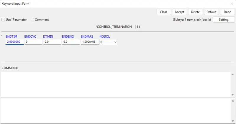
Keyword manager>CONTROL>TERMINATION
The control termination function is enabled to specify the end time of the simulation. The
termination time is set for 2 ms to capture the effect of the crash box striking the rigid wall.
DATABASE OPTION:
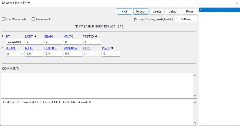
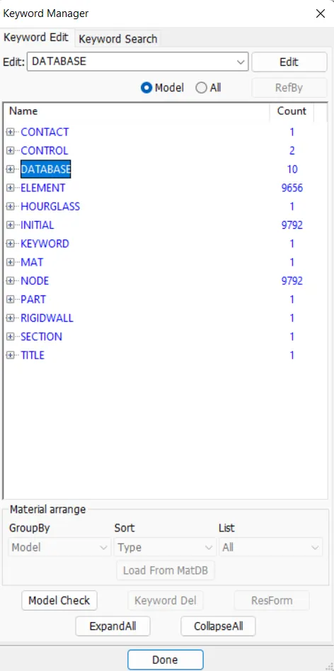
Keyword manager>DATABASE>BINARY_D3PLOT
The time step value of 0.02 ms is given for the BINARY_D3PLOT and in the
DATABASE_ASCII option for GLSAT, MATSUM, NODOUT, RCFORC, RWFORC,SECFORC and
SLEOUT.
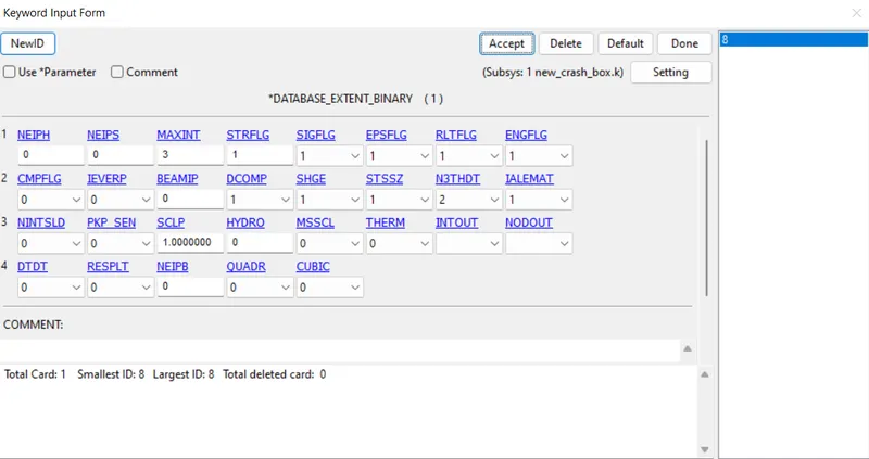
Keyword manager>DATABASE>EXTENT_BINARY
DATABASE_EXTENT_BINARY card with STRFLG =1, is used to compute the elastic strain in the model.
manager>DATABASE>HISTORY_NODE
DATABASE_HISTORY_NODE card is used to compute the acceleration of a 5094 node in
the crash box FE model.
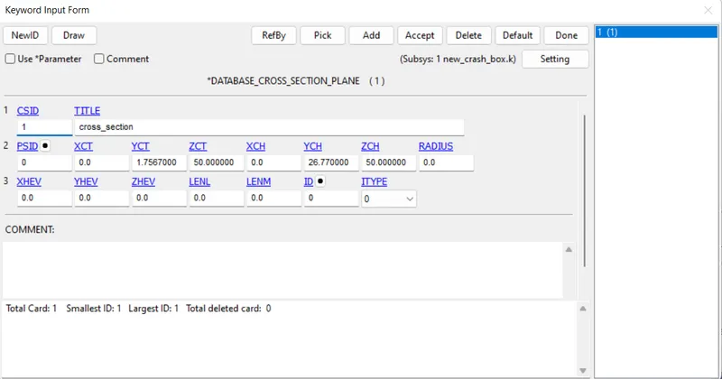
Keyword manager>DATABASE>CROSS_SECTION_PLANE.
DATABASE_CROSS_SECTION_PLANE card is used to compute the sectional force of the crash box.
Results:-The D3plot output File is opened in LS-PrePost using option File>open>LS-Dyna binary plot.
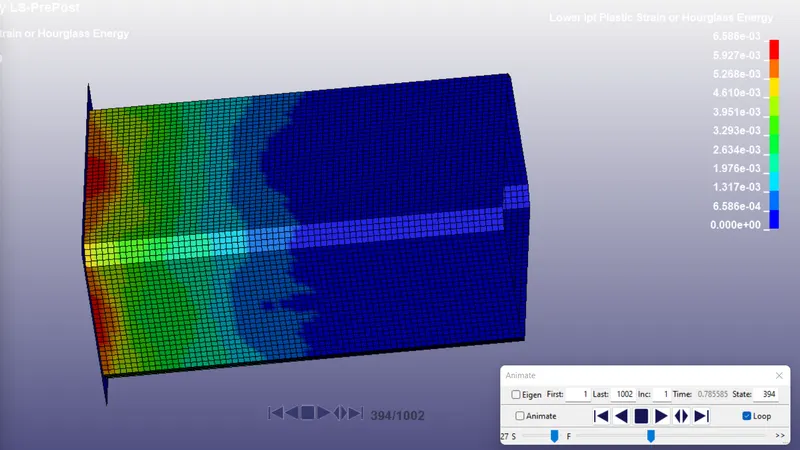
The animation of Von-Mises stress and Effective plastic strain for 1.2 mm and 1.5mm the thick crash box is shown below.
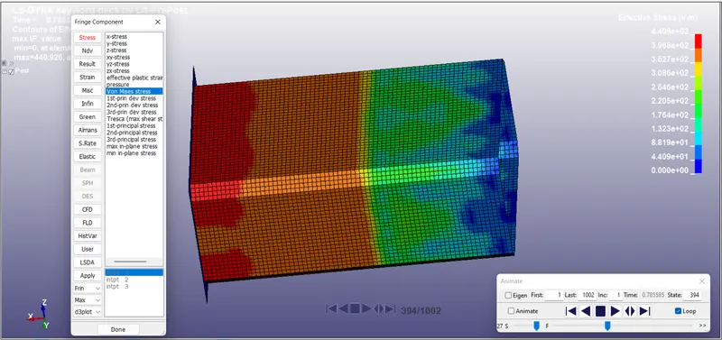
v-m stress animation contour of 1.2 mm thick crash box.
 .
.
Effective plastic strain contour of 1.5 mm thick crash box.
CONCLUSION:
1. The solver deck was set up for the crash simulation and the required results were
requested using the appropriate *DATABASE keyword cards.
2. The analysis ran successfully. Post-processing of the results was done using the D3plots
and the other output ASCII result files, to produce the deliverables.
3. The keywords necessary to build the crash box analysis was created from scratch.
1. The model was solved successfully and the results are compared for both 1.2 mm and 1.5
mm thick crash box.
2. The results of 1.5 mm crash box showed higher energy absorbing capacity and less
deformation compared to 1.2 mm thick crash
3. Learned to build a solver deck for simple crash analysis in LS-Dyna and extract the outputs
to interpret and compare the results.