Week 4 - CHT Analysis on Exhaust port

Introduction

Conjugate Heat Transfer (CHT) is applicable whenever there are two adjacent domains and we wish to analyse the heat transfer between these domains. These domains can either be solid or fluid domains

For many simulations of real world engineering applications, the predictions of heat transfer properties are as important, if not more important, than the actual flow field. Such scenarios include simulations of heat exchangers, HVAC (Heating, Ventilation and Air Conditioning), combustion/burners, electronics cooling, and many more. In these applications, we are often interested in how heat moves through both the fluid and solid domains, and importantly the transfer of heat across the interface between adjacent domains.

One example is the forced or natural convective cooling of a heat-sink attached to active electronics components which generate heat.

As well as heat-transfer across solid-fluid domains, we can also resolve heat transfer across solid-solid domains and fluid-fluid domains. Solid-solid interfaces are used where two solid components are in contact with each other and there is heat flowing between the objects. Although a fluid-fluid CHT system may seem unphysical, it is a valid assumption in some cases, such as a co-flow heat-exchanger where two fluids are separated by a thin wall. In this case, it can be assumed that the heat-transfer across the dividing wall is calculated in the wall normal dimension only (without explicitly meshing the wall thickness), and there is negligible heat flow along the wall.

In all of the above instances, a thermal resistance can be applied to the interface in ANSYS CFD. Such resistances can be used to represent thermal coatings (often used in electronics applications) or badly mated surfaces between adjacent solids (to understand the tolerance of poorly designed connections).

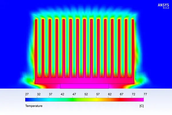
This image shows a cross-section through the stream-normal plane of the above finned heat exchanger. Heat flows into the heat sink from the active electronics components on the base and is carried through the heat sink fins and into the surrounding air. The boundary layer is critical to this heat transfer and an appropriate near-wall mesh is needed

In this project we are analysing the conjugate heat transfer through an exhaust port

Load the Cad file in space claim

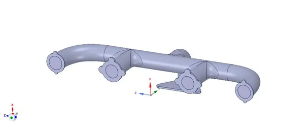
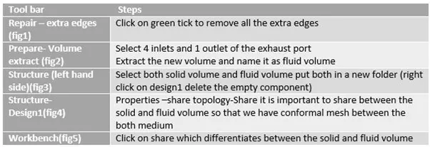
Fig 1

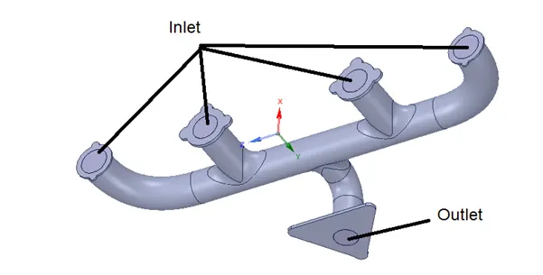
Fig 2

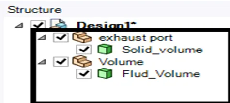
Fig 3

Fig 4

Fig 5

Meshing

Step1

After importing exhaust port in meshing Name the faces of each Face and then press keyword ‘n’By choosing Face icon

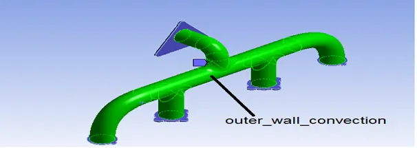
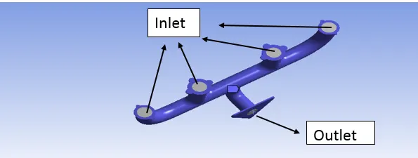
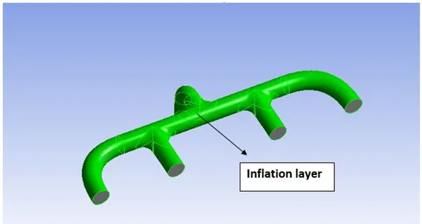
Step 2: Click on mesh –Detail mesh-Search for Inflation Then provide data

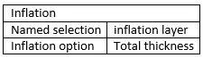
Step 3

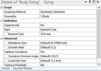
Mesh right click-sizing choose the solid body and mention the element size

Calculation of y plus

R_e=ρuL/µ= (1.225*5*150*10e-3)/ (1.7894*10e-5),

ρ, µ-properties of hot fluid coming towards exhaust port

u-velocity of hot fluid

C_f=0.079*R_e^ (-0.25) =0.0052481;

τ_w= (C_f ρ u² )/(2)=0.080361;

u_T= [(τ_w)/ (ρ)]^0.5=0.2314;

Y⁺= (ρ*u_T*∆y)/µ;

We will find ∆y considering Y⁺=30 (we are considering standard k-epsilon function so y⁺ value should be greater than 30 i.e it should lie in log region )

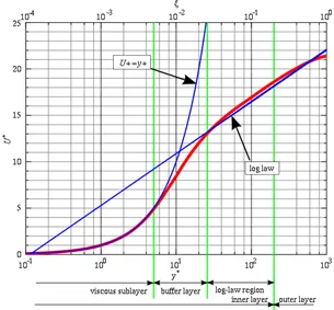
∆y=1.893665mm;

Considering 5 layers, with 20% growth in each layer

S₅=1.8936*(1-1.2⁵)/ (1-1.2) =14.0914mm

Setup:

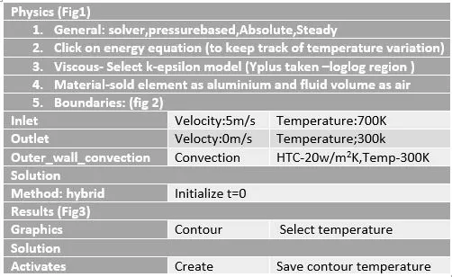
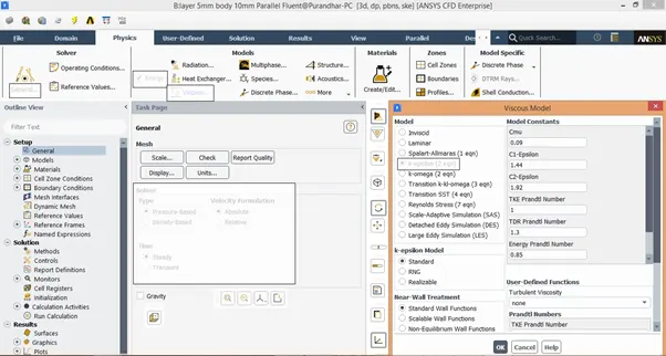
Fig1

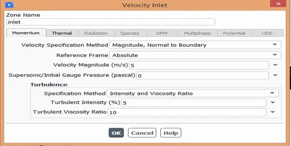
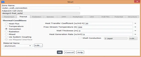
Fig2

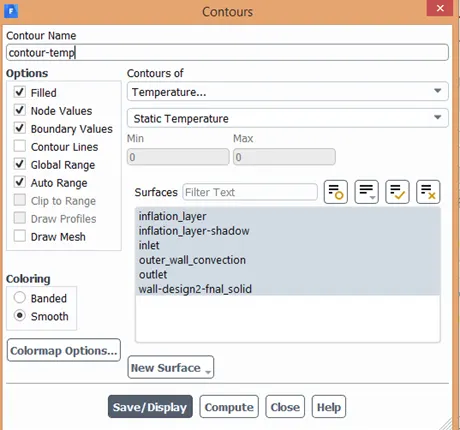
Fig3

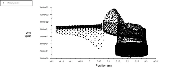
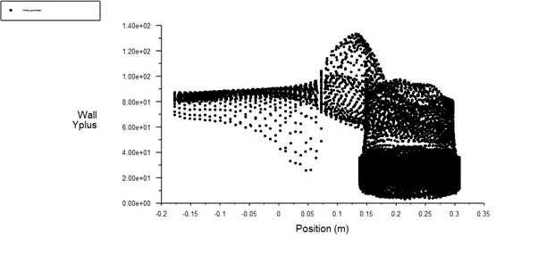
Maintaining the y+ value according to the turbulence model

Case1: Mesh elements 1060173 (meshing solid volume only)

Case2: Mesh elements- 1012088(meshing both sides sold and fluid volume)

Case3:Mesh elements-1212549(meshing both sides sold and fluid volume)

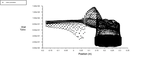
Both the plots are all most similar yplus lying between 30-140 in accordance with region k-epsilon model but few are below yplus of 30 lying in unconditional region which are there because of complexity of the geometry ,in order reduce this higher mesh resolution should be provided

Results of Case1 and Case3

Velocity

Case1

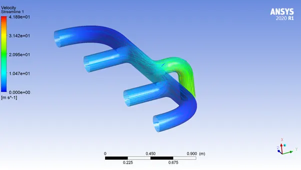
Velocity stream lines

Case1

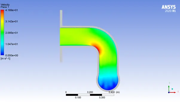
Case3

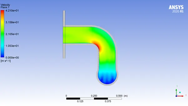
From continuity equation

We have A₁V₁=A₂V₂ formula implies for a fluid flow in a pipe

In A₁V₁+ A₂V₂+A₃V₃+A₄V₄=A₅V₅;

We consider that the 4 inlet are and exhaust port area are almost equal so the area cancels out

Therefore V₅> (V₁+V₂+V₃+V₄+V₅),

So velocity at exhaust will have higher velocity seen above in stream lines

Tempearture

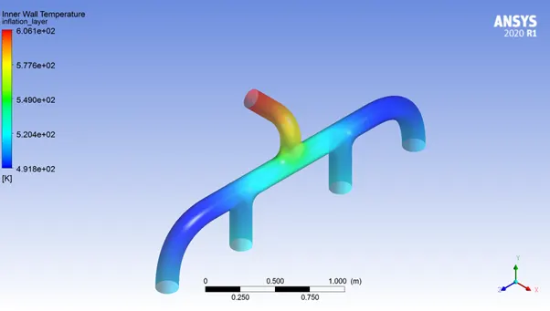
Case1

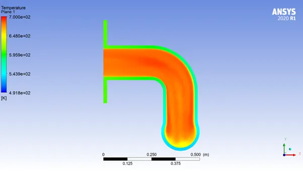
Case3

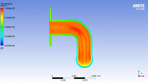
Temperature distribution at exhaust port

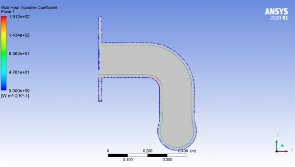
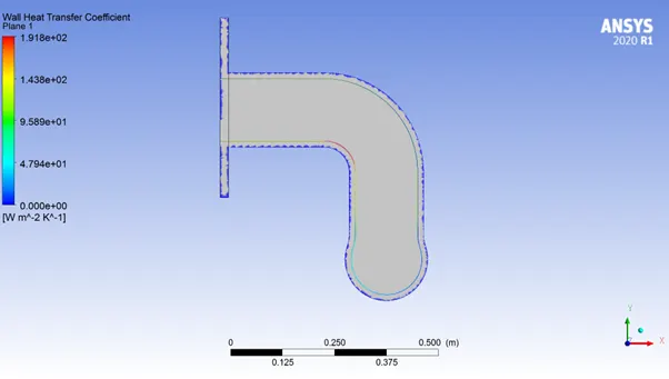
Heat transfer co-efficient at exhaust port

Case1

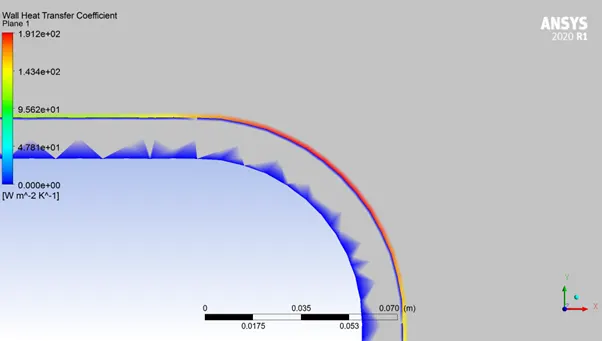
Case3

Verification of heat transfer co-efficient results from simulation

Numerical it can be done by calculating Nusselt number and heat transfer co-efficient

Nu = (convective heat transfer co-efficient)/ (conductive heat transfer coefficient)

=hL/k;

Nu-(Re, Pr), here Nusselt number is function of both Reynold’s and Prandle’s number

Given by Nu=0.023*Re^0.8Pr^0.3 (Dittos’ Boelter Equation)

Where we find Nu number Re and Pr can be easily calculated by knowing the fluid property, then Nu is substituted in first equation h of fluid can be calculated numerically

Factors on which accuracy of prediction depends

• Finer the mesh better will be the accuracy of heat transfer co-efficient of the fluid
• Depends on selection of turbulence models ,the plus in the inflation layer should be in according to turbulence model and most of cells should lie in favourable zone (turbulence model)

Conclusion:

1. Choosing Yplus in accordance with turbulence model plays vital role in determining the heat transfer co-efficient of the hot gases
2. Inflation layer should contain an optimum layer to determine heat transfer co-efficient effectively