Week 4 - CHT Analysis on Exhaust port
Aim:
To carry out the Conjugate Heat Transfer analysis of Exhaust Port.
Objective:
After preparing the geometry in the Ansys Spaceclaim, carry out the simulation in Ansys Fluent to determine the velocity & temperature distribution inside the exhaust port. Following are the main objective that are required to present into the report:
- Give a brief description of why and where a CHT analysis is used.
- Maintain the y+ value according to the turbulence model and justify the results.
- Calculate the wall/surface heat transfer coefficient on the internal solid surface & show the velocity & temperature contours in appropriate areas.
- How would you verify if the HTC predictions from the simulations are right? On what factors does the accuracy of the prediction depend on?
Model Preparation:
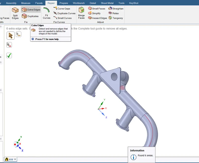
First of all Exhaust port model has been imported into the Spaceclaim to prepare it for the simulation. Some extra edges has been found into the model which has been identified using the "Extra Edges" command available in the "Prepare" tab of Spaceclaim. 6 extra edges were present into the model which have beed shown into the followiing image with the location of the command. The edges have been removed using the same command.
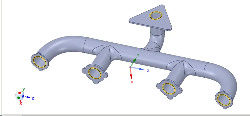
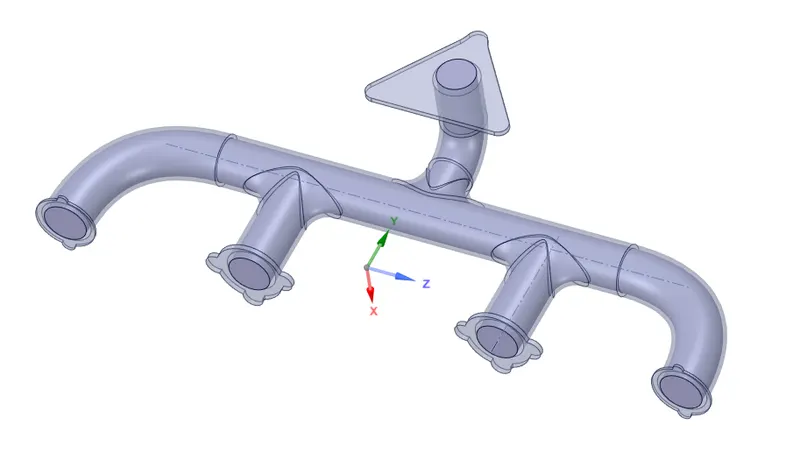
The fluid volume has been created using the volume extraction command. In first image, the edges has been selected to define the close volume. And in second image, the extracted volume has been shown.
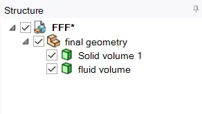
The fluid & solid domain were placed in two seperate components. Both domains has been brought together in single component as shown in the following image.
To create interface between the fluid volume & solid volume of the exhaust port body, the shared topology is required to create. Without shared topology, especially in CHT analysis, the heat transfered from the fluid to the solid or vice versa will not be accurate. And without shared topology, mesh has been developed at the interface without proper alignment of the elements which is called the non conformal mesh. Following image shows the similar phenomena.
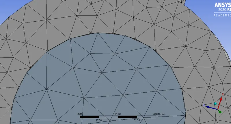
To accurately simulate the CHT analysis, conformal mesh is required to create and by creating shared topology, this problem can be solved.
First of all, the shared topology option has been slected for the component.

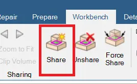
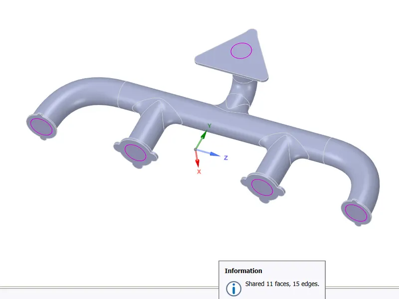
And using the option called "Share" commad from the sharing panel needs to be executed to complete the process of sharing the topology & developing common interface between fluid & solid domain. In second image, pink edges shows the confirmation of successfully created shared topology.
After executing shared topology process, the mesh has been recreated which is shown in following image. The mesh element between the fluid & solid domain are aligned very accurately.
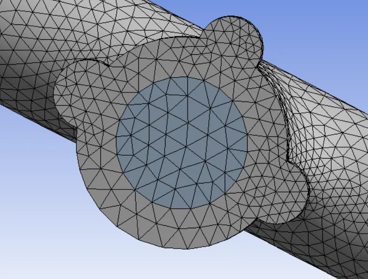
The inflation layers has been created by mainting the y+ values. The calculation for first layer thickness & total layer thickness has been shown in detail in following section.
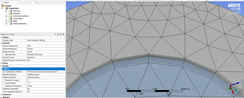
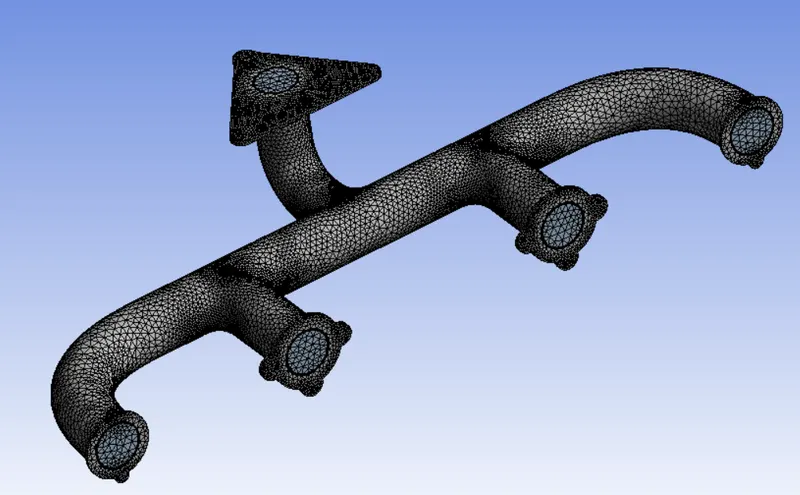
Final mesh has been shown in the following image.
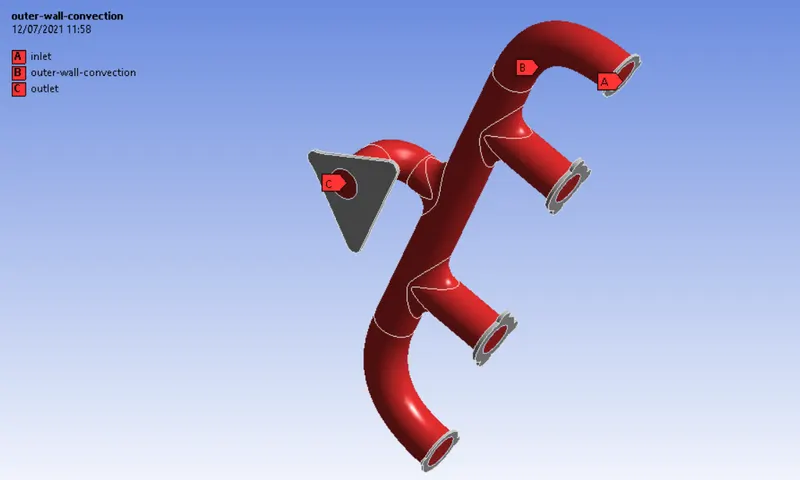
Following faces have been given name to identify easily during simulation setup.
Simulation Setup:
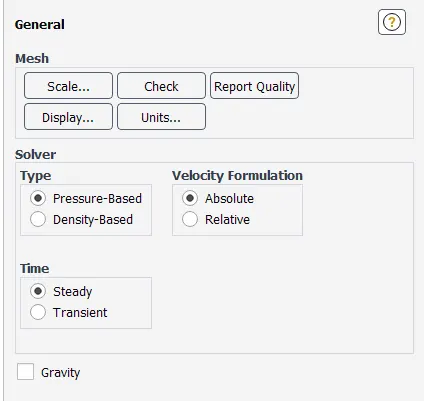
The simulation will be carries out using pressure based solver with steady state condition.
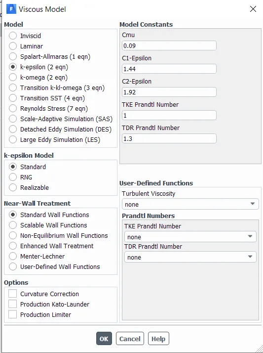
k-epsilon with standard near wall treatment option has been selected from viscous model dialogue box. Energy eqaution has been turned on for this simualtion.
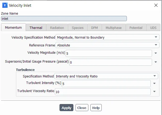
The inlet condition will be set as per following image with air temperature set as 700 K (426 degree celcius). Outlet has been set as pressure outlet with gauge pressure equal to 0 Pa.
20 W/m^2.K heat transfer coefficient has been given to the outer wall using convection option.
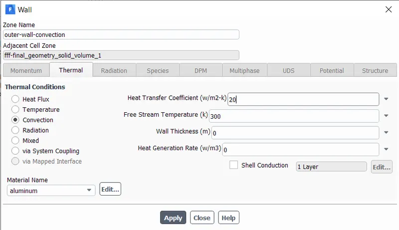
Deafult material has been taken for the simulation. Air for the fluid & aluminium for the exhaust port.
After selecting Hybrid method for the initialization, the simulation has been initialized & 150 iterations has been fixed for the solver to determine the solution. Results has been shown in following section.
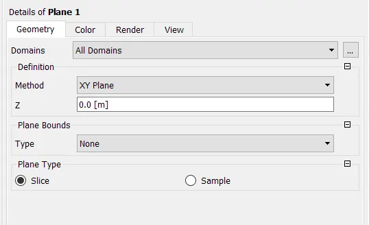
During post processing, planes are created to understand velocity & temperature districbution inside the exhaust port.
First plane has been created parallel to XY plane while the second plane has been created 0.22m offset to YZ plane.
Q & A:
1. Give a brief description of why and where a CHT analysis is used.
CHT analysis means Conjugate Heat Teansfer analysis. The CHT analysis has been performed when the heat transfers from the solid domain to fluid domain or vice versa through the interface between two states. The applications of CHT analysis are heat transfers, cooling of electronic products and general heating & cooling systems.
2. Maintain the y+ value according to the turbulence model and justify the results.
In current simulation, the total height of the inflation layer has been set as 5 mm.
Now, following is the cross-checking of inflation layer thickness by calculating y+ which is dimensionlesss number.
In turbulent flows, the flow nearer to the wall is laminar for very small region if the wall has no-slip condition has been given.
y+ value will help the designer to understand how coarse or fine the generated mesh is for particular method. As per boudary later theory, the y+ value for the viscous sublayer would be less than 10 and if were modeling for the turbulent region, than the y+ value would be greater than 30.
So for this problem, the value of y+ will be taken as 10.
The equation of y+ is :
`y+ = (y*u^**)/nu`
where, y = distance from the wall in mm
`u^**` = friction velocity in m/s
`nu` = kinematic viscocity in kg/ms
The friction velocity can be defined as the velocity of the flow in the region near to a wall. It can be calculated using following formula:
`(u^**)^2 = tau/rho`
so, `u^** = sqrt(tau/rho)`
here, `tau` = wall shear stress in Pa = `0.5*(Cf * rho * u^2)`
where, u = free stream velocity in m/s
and, `Cf` = skin friction coefficient which is defined as The skin friction coefficient is an important dimensionless parameter in boundary-layer flows. It specifies the fraction of the local dynamic pressure that is felt as shear stress on the surface.
`Cf = 0.0576*Re^(-1/5)`
where Re = Reynolds Number
`Re = (rho*u*L)/mu`
where = rho = fluid density in kg/m^3
u = free stream velocity in m/s
L = characteristic linear length in meter
`mu` = dynamic viscocity of fluid in kg/ms
So, for this problem,
u = 5 m/s
L = 0.166 m (Inlet port dia has been considered)
`mu` = 1.7894e-5 kg/ms
`rho`= densty of air = 1.225 kg/m^3
Now, calculating Re first.
Re = (1.225 * 5 * 0.166)/1.7894e-5 = 56820
Skin frinction coefficient =`Cf` = 0.0576 * 56820^(-1/5) = 0.00645
Wall Shear Stress = `tau` = 0.5*0.00645*1.225*5^2) = 0.0988 Pa
Now, frinction velocity, `u^**` = sqrt(0.0988/1.225) = 0.28 m/s
So, distance from the wall, y = (10*1.7894e-5)/0.28 = 0.00063 m = 0.63mm
The value of y here shows the distance from the wall to the first node. In finite volume method (FVM), the node is the centroid of the first element. So, following table shaws the calculation of the total inflation layer thicknes to capture the flow characteristics in the laminar region. 20% growth has been given from the first layer onwards. Thats why each layer thickness has been increased 20% from the last layer.
| Layer Growth Rate | 1.2 | |
| Distance from the wall (y) | 0.63 | mm |
| 1st Layer (2*y) | 1.26 | mm |
| 2nd Layer | 1.512 | mm |
| 3rd Layer | 1.8144 | mm |
| 4th Layer | 2.17728 | mm |
| 5th Layer | 2.612736 | mm |
| Total Thickness | 9.376416 | mm |
So, the total inflation layer thickness considered in the simulation of 5 mm is below the maximum allowable total thickness as per analytical method shown in the above table.
3. Calculate the wall/surface heat transfer coefficient on the internal solid surface & show the velocity & temperature contours in appropriate areas.
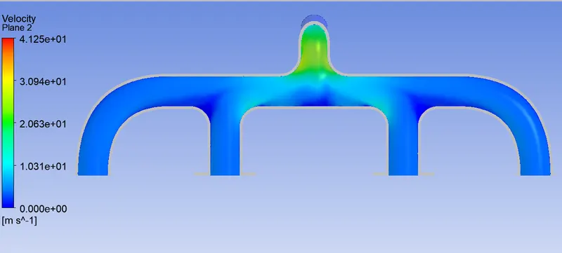
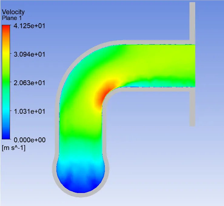
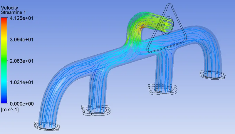
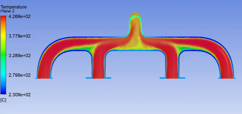
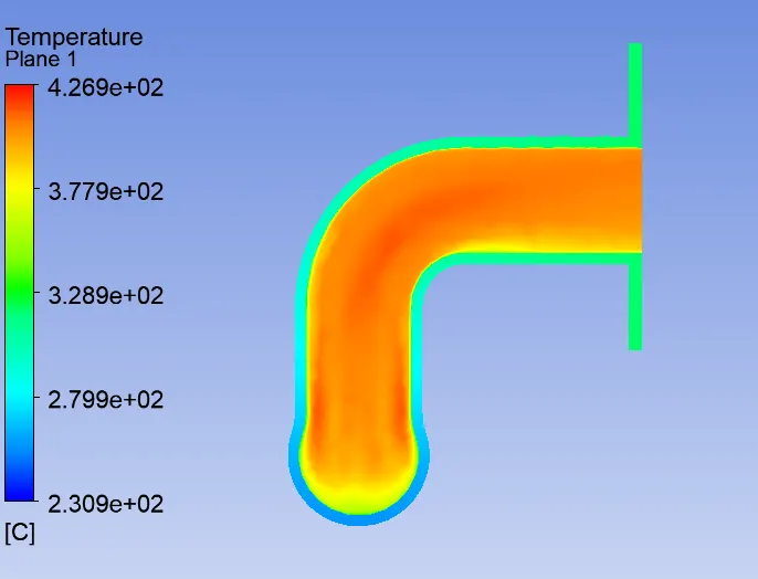
In first two images, the velocity contours has been projected on both reference planes while in the thrid image, streamlines has been used to understand the air velocity profiles inside exhaust port. Later, in similar way, temperature distibution has been projected on both reference planes.
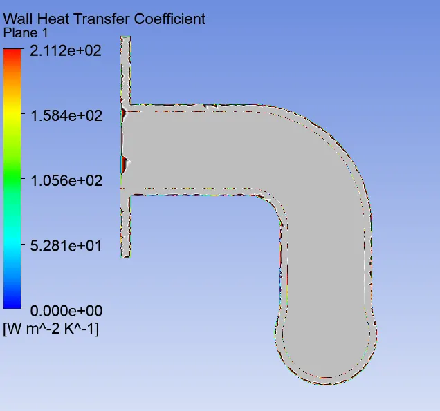
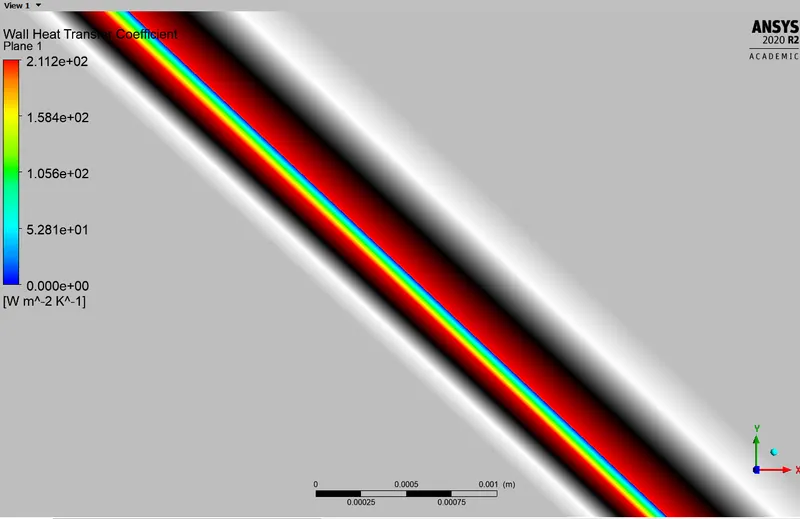
At last heat transfer coefficient near the wall has been displayed.
Velocity Contours:
Velocity Streamlines:
Temperature Contours:
Heat Transfer Coefficient:
4. How would you verify if the HTC predictions from the simulations are right? On what factors does the accuracy of the prediction depend on?
Heat transfer coefficient can be determined using the Nusselt Number (Nu) equation, which is
`Nu = ("Convective Heat Transfer")/("Conductive Heat Transfer") = (h*L)/k`
where, h = convective heat transfer coefficient in W/m^2.K
L = characteristic diamerer in meter = 0.166m
k = thermal conductivity in W/m.K = 0.0242 W/m.K
To determine, Nusselt Number, the Dittus-Boeltr equation for internal turbulent flow condition will be used which is,
`Nu = 0.023 * Re_(Dh)^0.8 * Pr^0.4`
where, Pr = Prandtl Number for the air with 700 K temperature = 0.71
Re = 56820
So, Nu = 0.023 * (56820)^0.8 * 0.71^0.4 = 127. 59
From first equation of Nusselt Number,
h = (Nu*k)/L = (127.59*0.0242)/0.166 = 18.6 W/m^2.K
So, the heat transfer coefficient consider for the simulation, which is 20 W/m^2.K, is very near by the calculated heat transfer coefficient. The calculated Nusselt Number's value depends on the Prandtle number & Reynolds number. And also, the Dittus-Boeltlr equation is accurate for the smooth circular pipe with small to moderate temperature differences and it is less accurate for rough pipes & large temperature variations. Because of these factors, the difference in the calculated heat transfer coefficient & coefficient consider for simulation is acceptable.
Results Discussion:
In second & third image of velocity distribution, the maximum velocity can be seen in the red color near the turining where pressure has been dropped due to sudden turn in profile & following to the maximum velocity area, low pressure area has been build up.
In similar way, in first image, the low pressure area has been seen in dark blue between the ports & low temperature can be seen at the same place in temperature distribution graph. The temperature starts dropping towards reaching the outlet of exhaust port because of the heat is transferring from the exhaust port walls & also the air from the low pressure areas in the exhaust port where air with less temperature mixed up with the hot air.
In last two images, the heat transfer coefficient has been shown. The heat transfer coefficient only visible in the first layer of the inflation layers. Thats why, in second image, the area has been zoomed to make it visible.
References:
1. https://skill-lync.com/knowledgebase/what-is-yplus
2. https://www.thermopedia.com/content/790/
3. https://www.simscale.com/docs/analysis-types/conjugate-heat-transfer-analysis/