Week 4 - CHT Analysis on Exhaust port

CHT analysis:

• Conjugate heat transfer analysis describes heat transfer as a result of interaction between a body and a fluid that is flowing over or inside it.

• At the matching interface, the details are provided for temperature distribution and heat flux along the interface eliminating the need of calculating the heat transfer coefficient. Moreover, the heat transfer coefficient can be calculated later.

• One of the simplest ways to realize conjugation is through numerical methods. The boundary condition for the fluid and solid interface is set and solved through iteration methods. There are no right guesses for the values of the initial boundary condition for the convergence except through the hit and trial method.

Application of CHT analysis:

• The CHT methods have become a more powerful tool for modeling and investigating natural phenomena and engineering systems in different areas ranging from aerospace and nuclear reactors to thermal goods treatment and food processing from the complex procedures in medicines to ocean thermal interaction in metrology.
• CHT in recent years has significantly improved the cooling performance of electronic equipment such as the design of heat sinks and the design of heat exchangers for the waste treatment plant. One such application of CHT is the exhaust port system.

Y+ value:

• To calculate the boundary values accurately, the mesh needs to be finer at the boundaries. The y+ value can be used to determine the mesh size to be used at the boundaries.
• It is a non-dimensional distance that is often used to describe how coarse or fine a volumetric mesh is for a flow pattern. The y+ is applicable only for turbulent flow and mesh cells directly in contact with a no-slip wall.
• The y+ values less than 5 are preferred for boundary layer problems, as the solver in the post-process uses viscous sublayer equations for those values.

SIMULATION PROCEDURES IN ANSYS WORKBENCH :

a) Geometry - Space Claim :

• First we have to import the geometry inside the space claim.

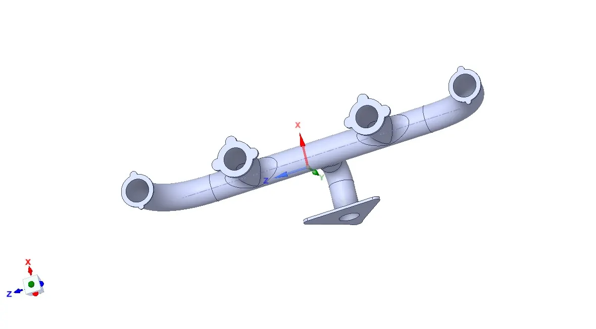
• The exhaust port is a three-dimensional model containing four inlets and one outlet.
• We have to change to meter in unit option inside space claim . We have to check any overlapping plane and lines are there by using Extra Edges inside this model. After geometrical clean up we are going to make inside solid by using volume Extract .With this solid we can use for future analysis .

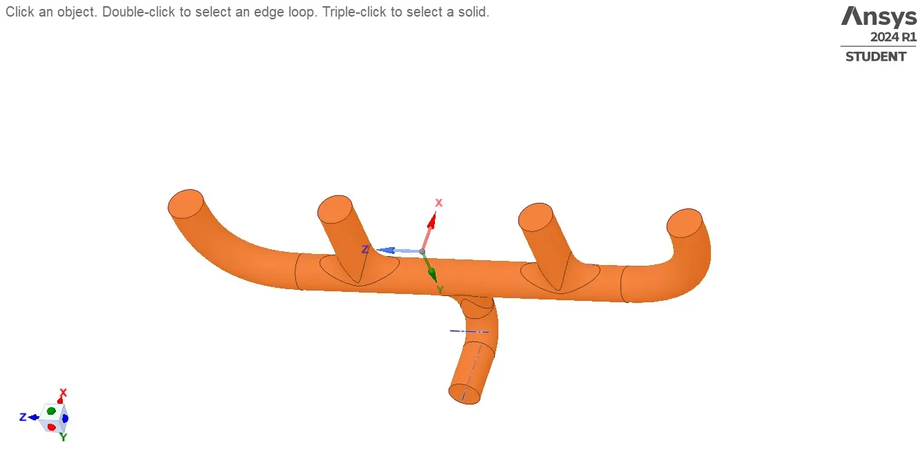
• Fluid volume is shown like this

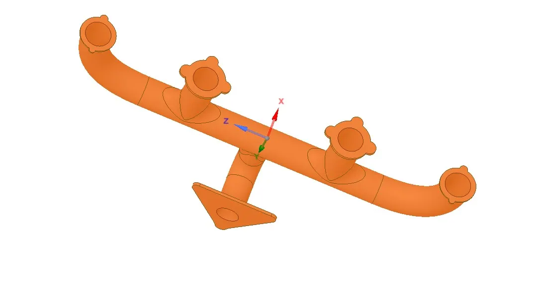
• Solid volume look like this

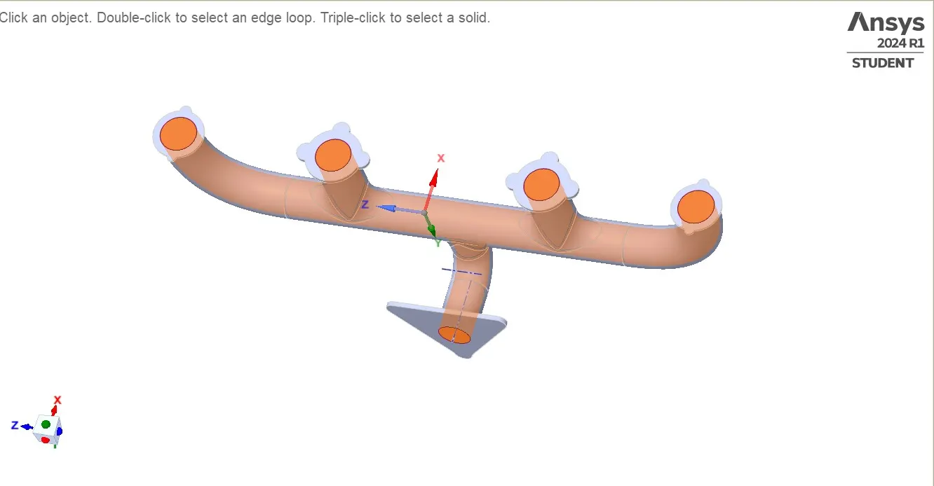
• CHT analysis consider the interplay between heat conduction in solids and fluids, and treats heat flux as continuous across the interface. That why we make it as both fluid and solid inside this model, it look like as

• We have to change to share in share topology because without this solid and fluid volume cannot share information between them.

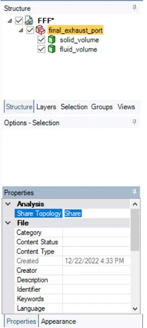
• We have to use the shareprep tools because after using this tool the solid and fluid volume can share the information.

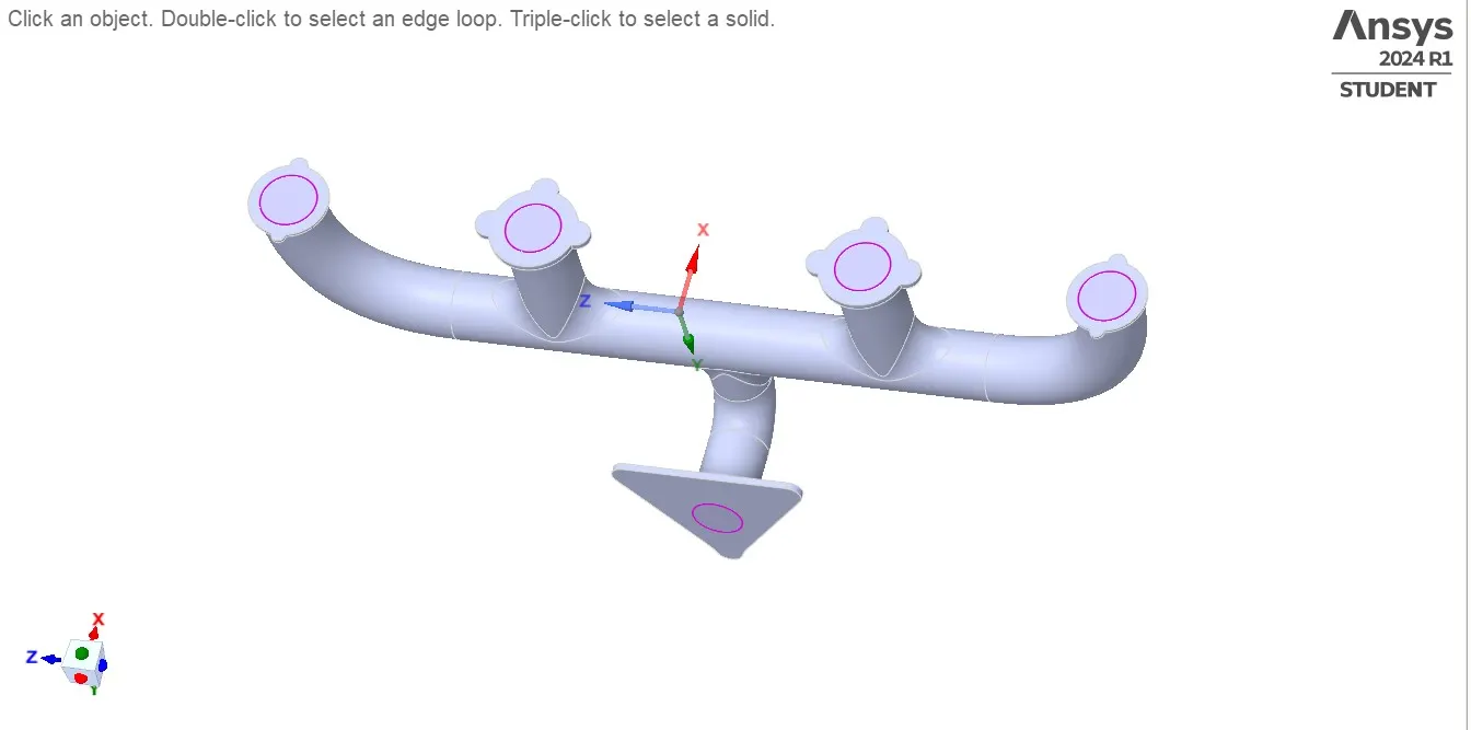
• We have to close the Geometry-space claim.

Mesh - Meshing :

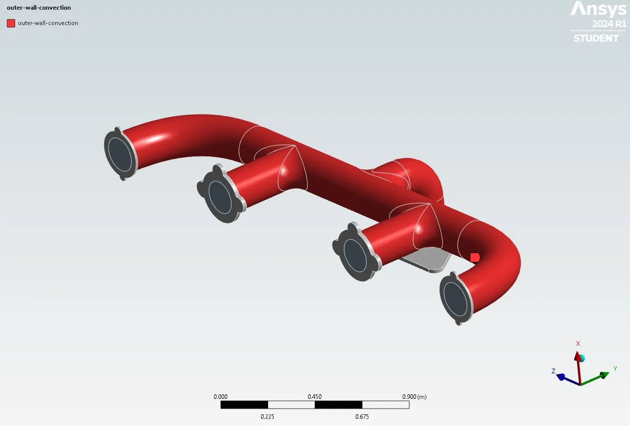
• We have to make name selection before going to meshing which is Inlet , Outlet and Outer wall convection.

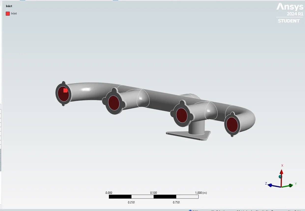
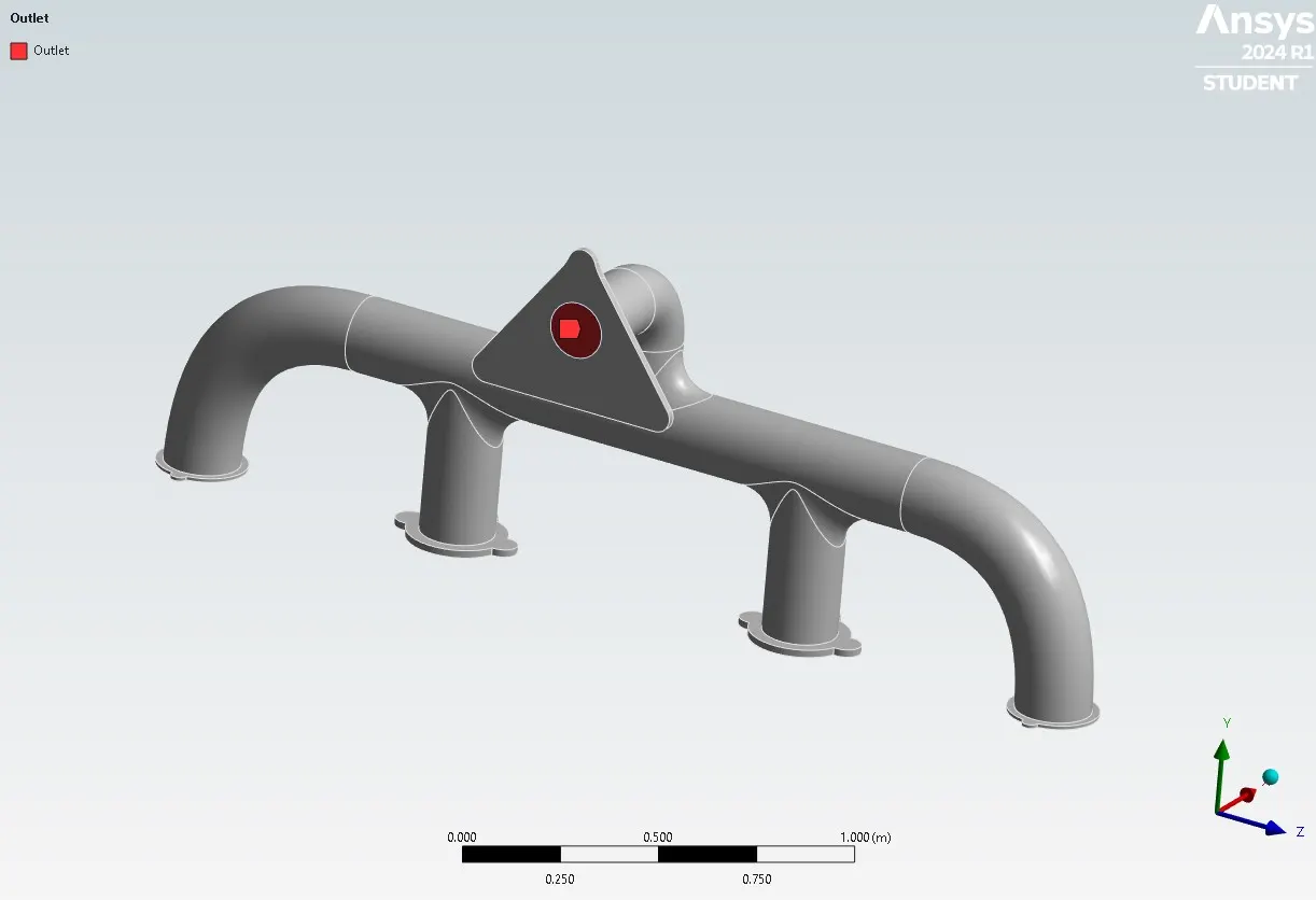
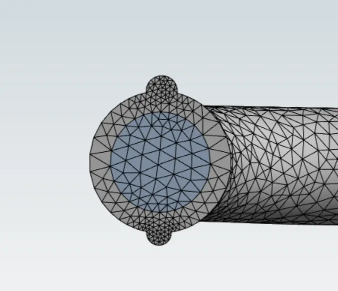
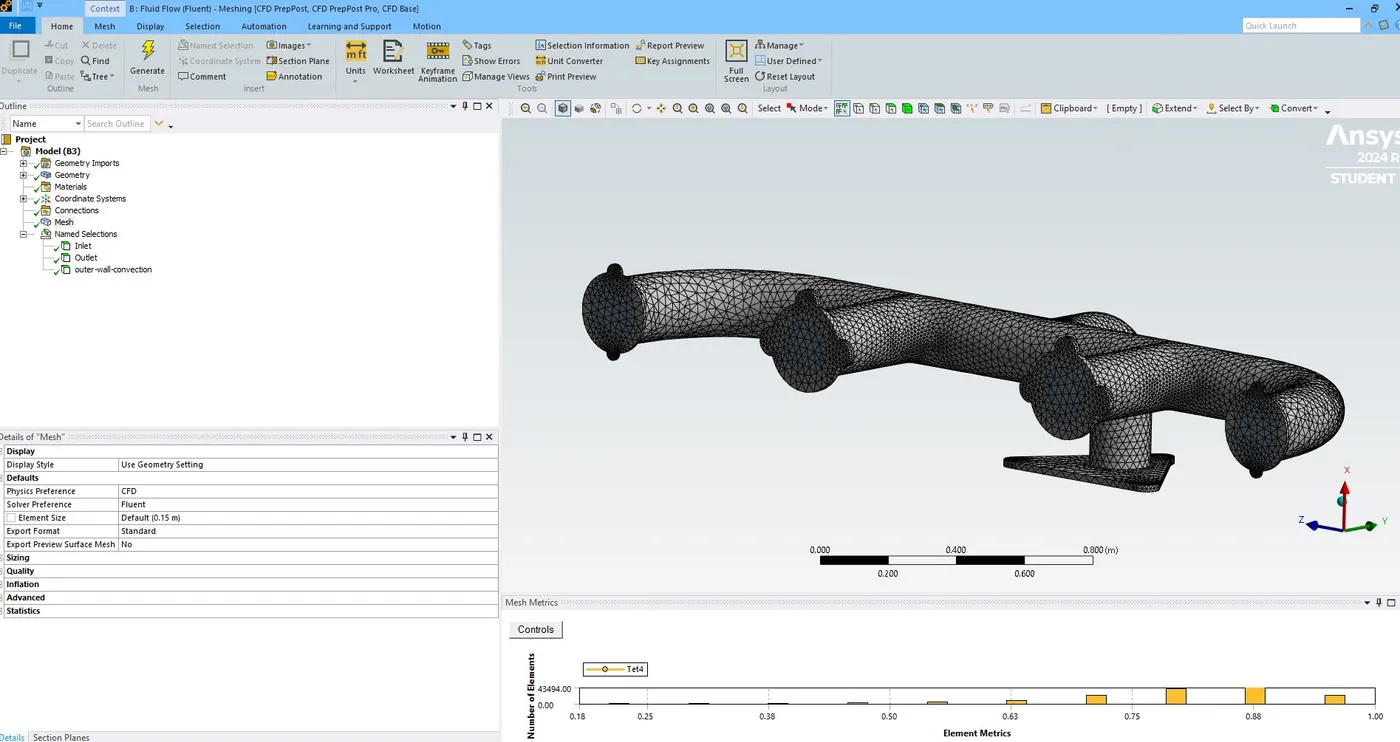
• We are going to mesh entire model with default mesh size is 150mm. check if the mesh from solid and fluid volumes are in sync. The mesh quality checked.

Setup - Fluent

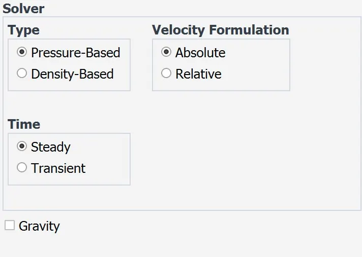
• The mesh geometry loaded in Ansys fluent. We have used pressure-based solver in type for this simulation and also we have run with steady State for this simulation

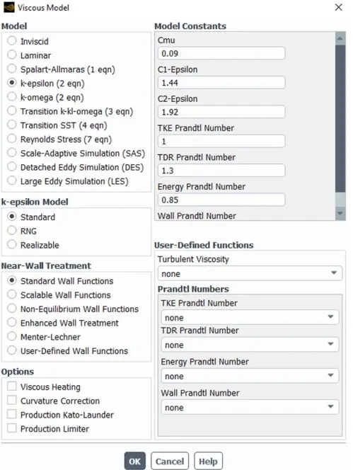
• We are going to include energy equation then For this simulation we are going to use K-Epsilon .

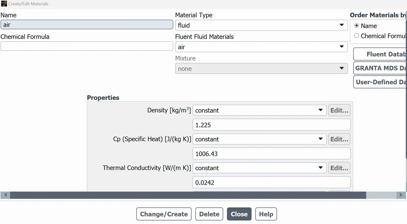
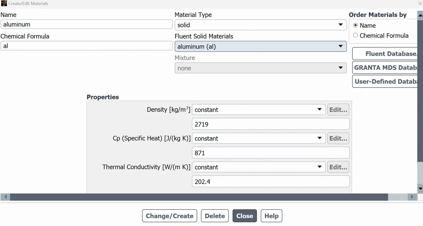
• After that we have to go inside materials and we are using default materials which is Air used in Fluid type and Aluminum in solid type.

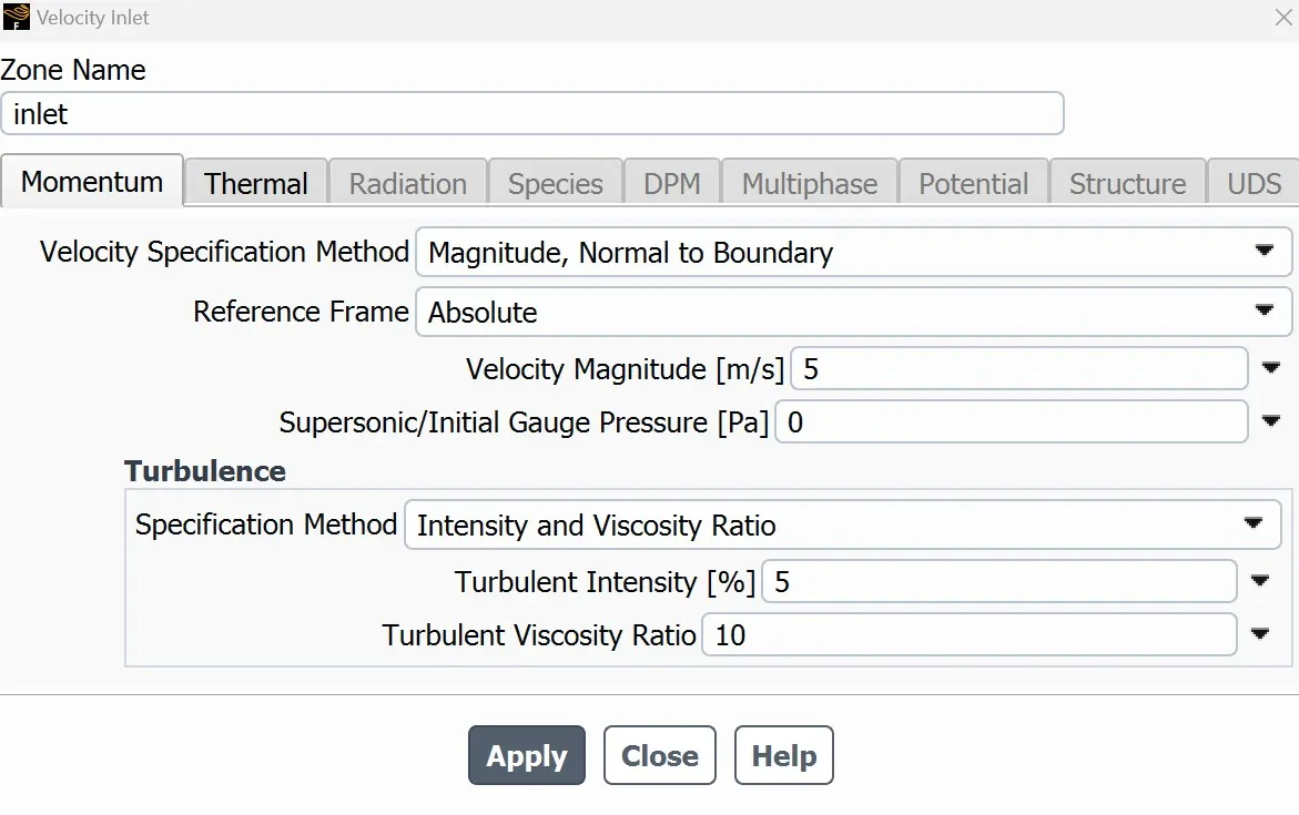
• We have to go inside Boundaries then we have to give the velocity is 5m/s and temperature is 700k.

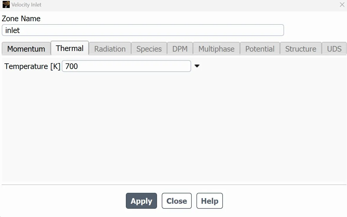
• The outlet is a pressure boundary.
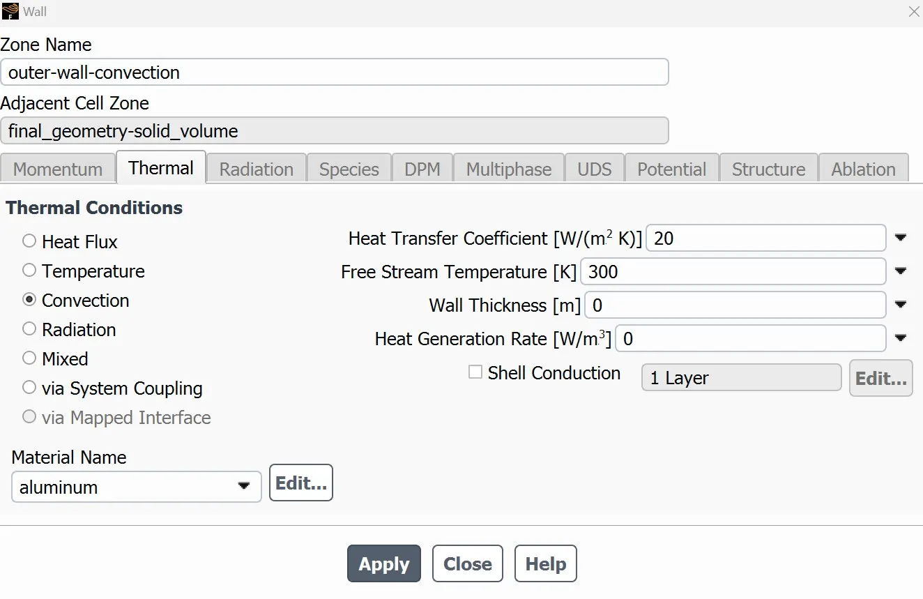
• In thermal condition , we have to used the convection and the heat transfer coefficient is 20 and temperature is 300k.
• The heat transfer coefficient for the outer wall, h = 20 W/(m2k) is assigned after verifying with analytical value.

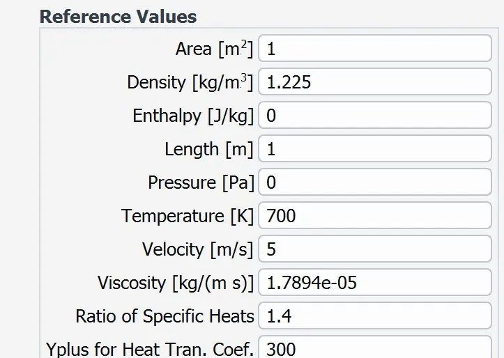
• We are going to put value inside the reference value ,

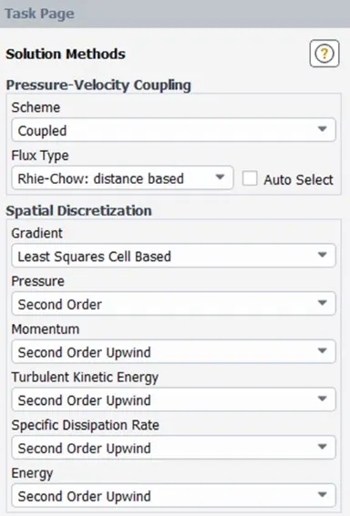
• We are going to use solution method for this simulation. Then we have to change to couple option inside scheme.

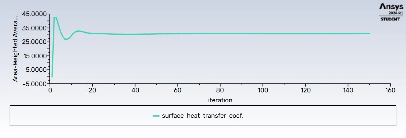
• In Area weighted average ,we need to measure the surface heat transfer coefficient inside the surface of pipe.

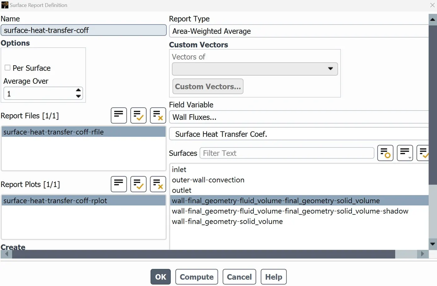
• We are going to initialize the hybrid initialization for making the temperature contour.
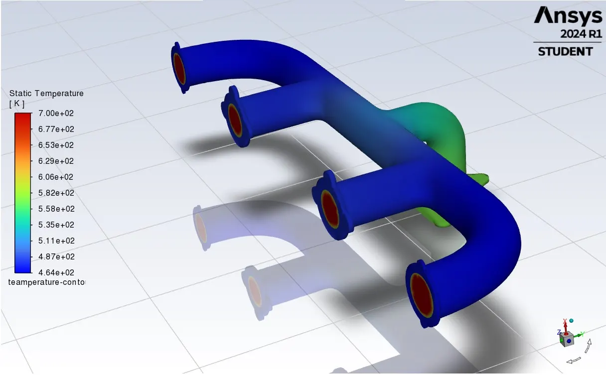
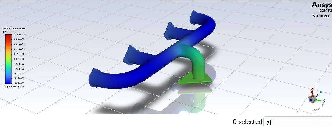
• Then the temperature contour is done and also solution animation is created.

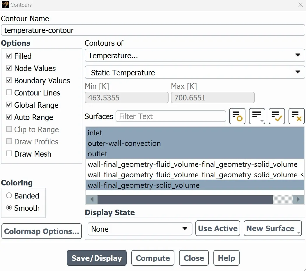
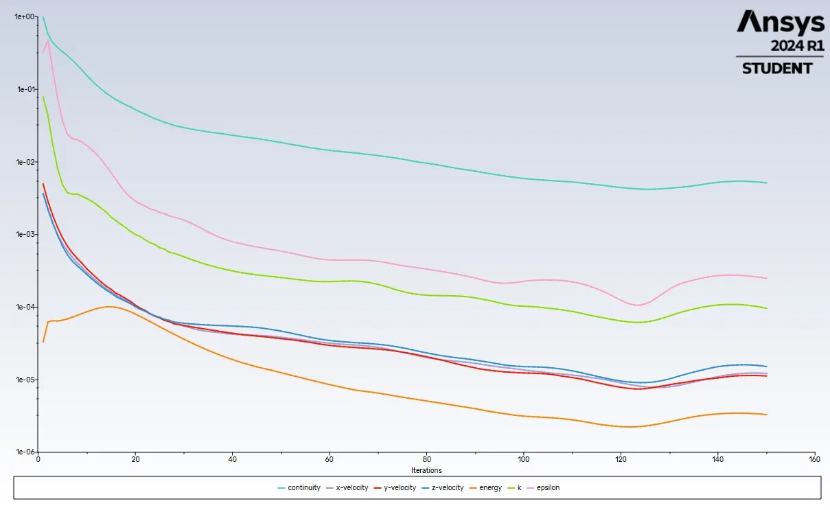
• We are going to calculate 150 iteration inside the run calculation.
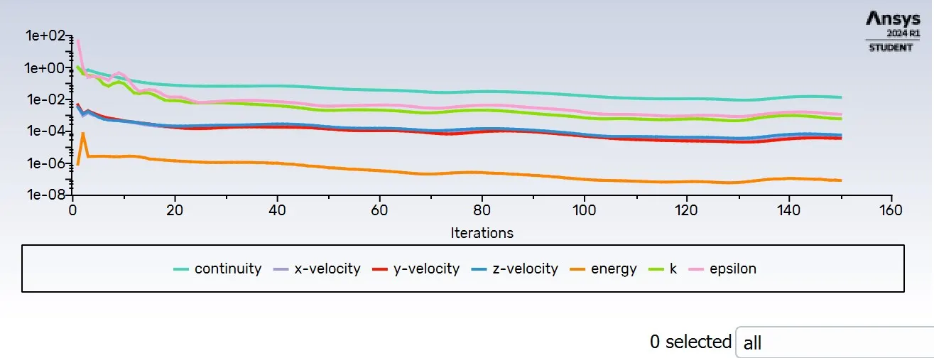
• After that i will got residual plot, temperature contour plot and surface heat transfer coefficient. It shown like this,

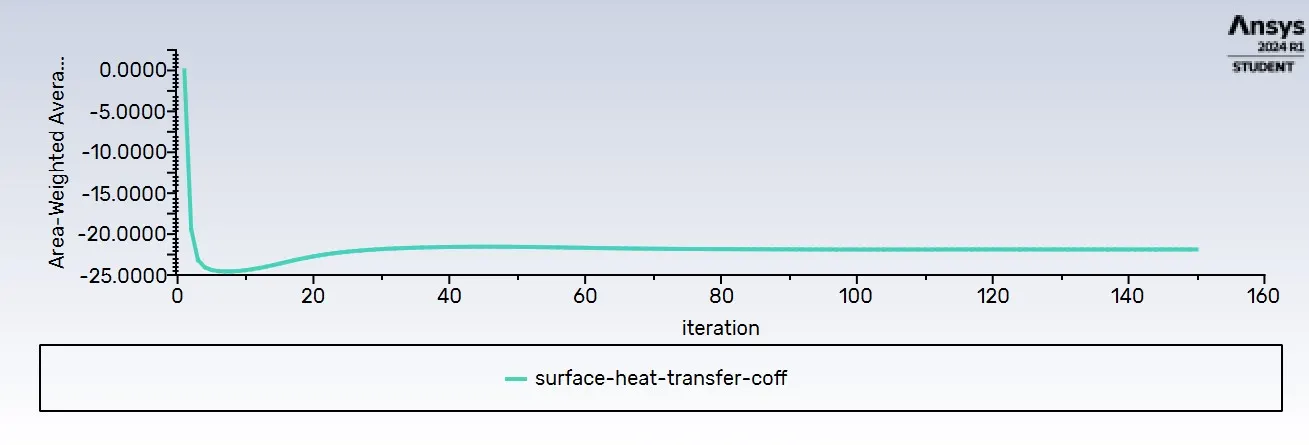
• We need to compute the surface heat transfer coefficient then we will got result.

• The outer wall which is outer wall convection also calculated .

• We have to exit from setup .

Result-Post processing

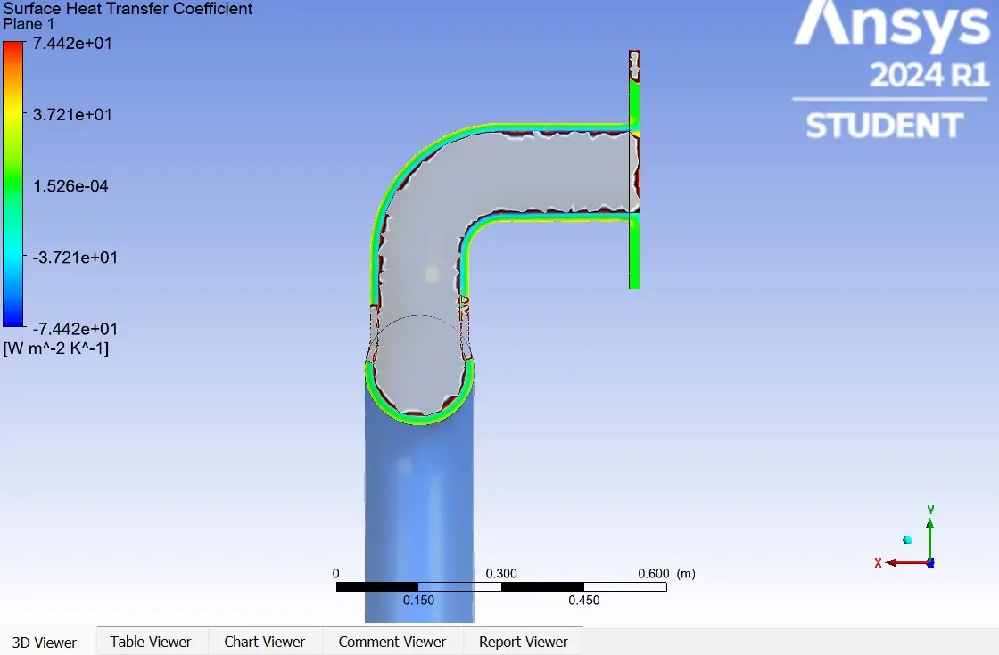
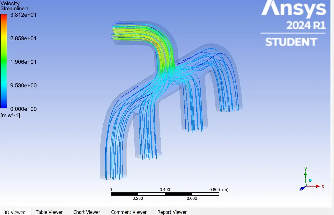
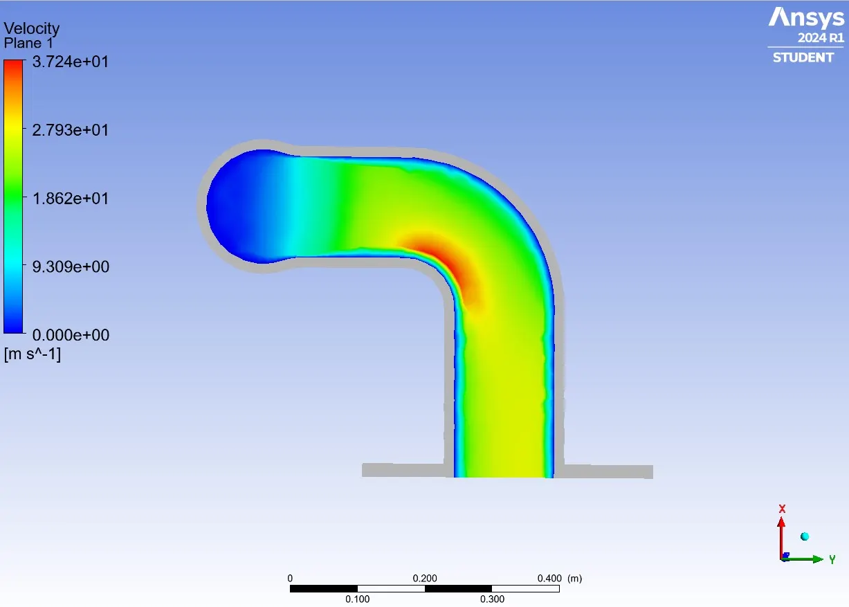
• We are going to make surface heat transfer coefficient and velocity streamline plot.

Refined mesh (K-Epsilon model) :

Geometry-Space claim

• • The geometry is the same as the baseline simulation.

Mesh-meshing

• We are added extra extra name selection for creating the inflation layer.
• The inflation layer boundary is the outermost layer of the fluid volume which is selected by hiding the solid surface.

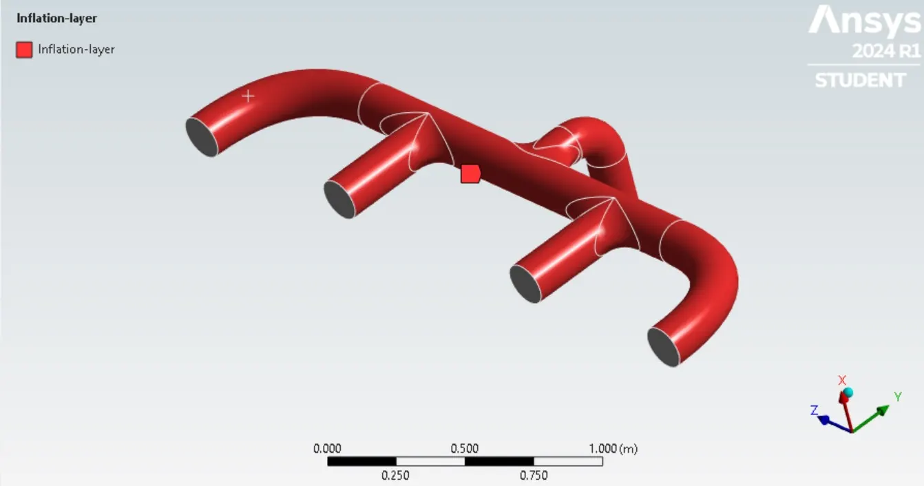
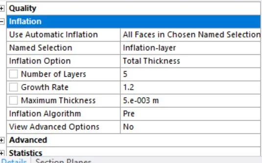
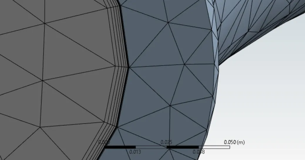
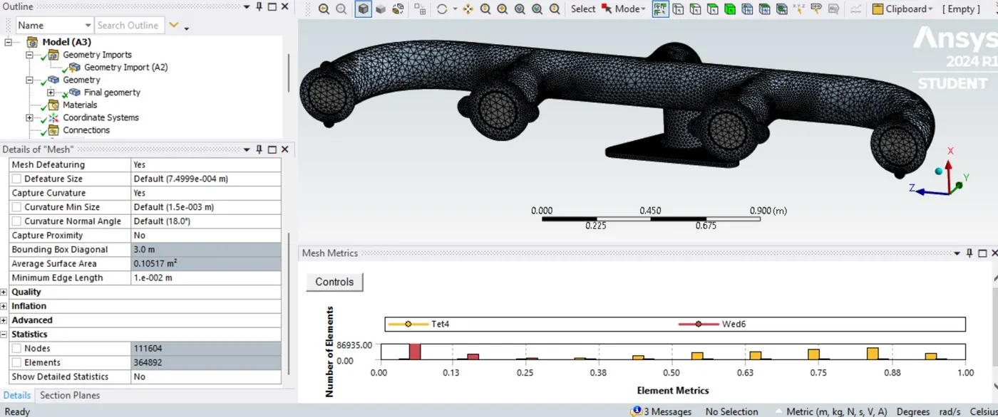
• The inflation layer is created below.

Setup :

• The K-Epsilon is used inside the turbulence model.

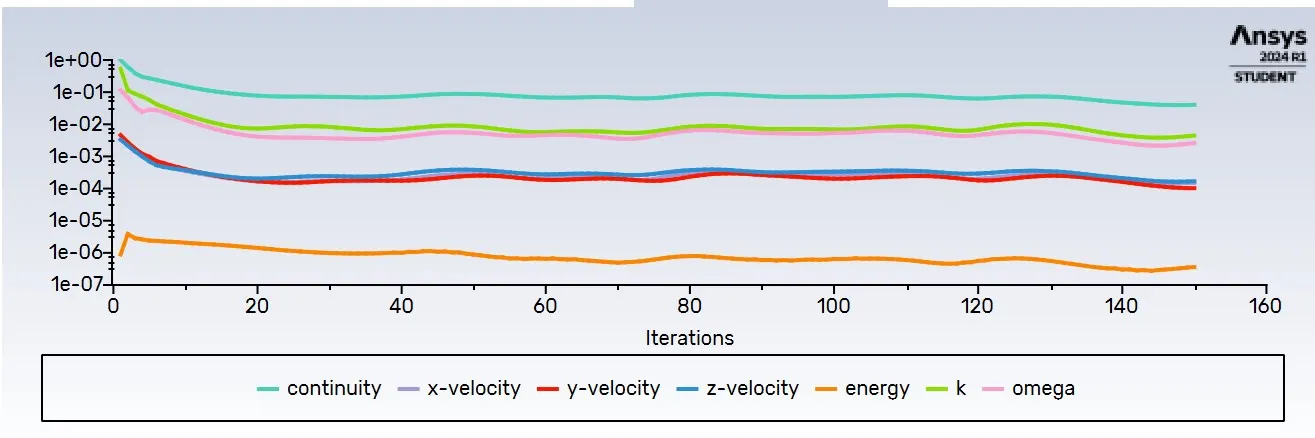
Result of Residual plots:

Temperature contour:

Surface Heat Transfer Coefficient:

• We need to compute the surface heat transfer coefficient then we will got result.

• Also we have to compute the outer wall.

Refined mesh (K-Omega model) :

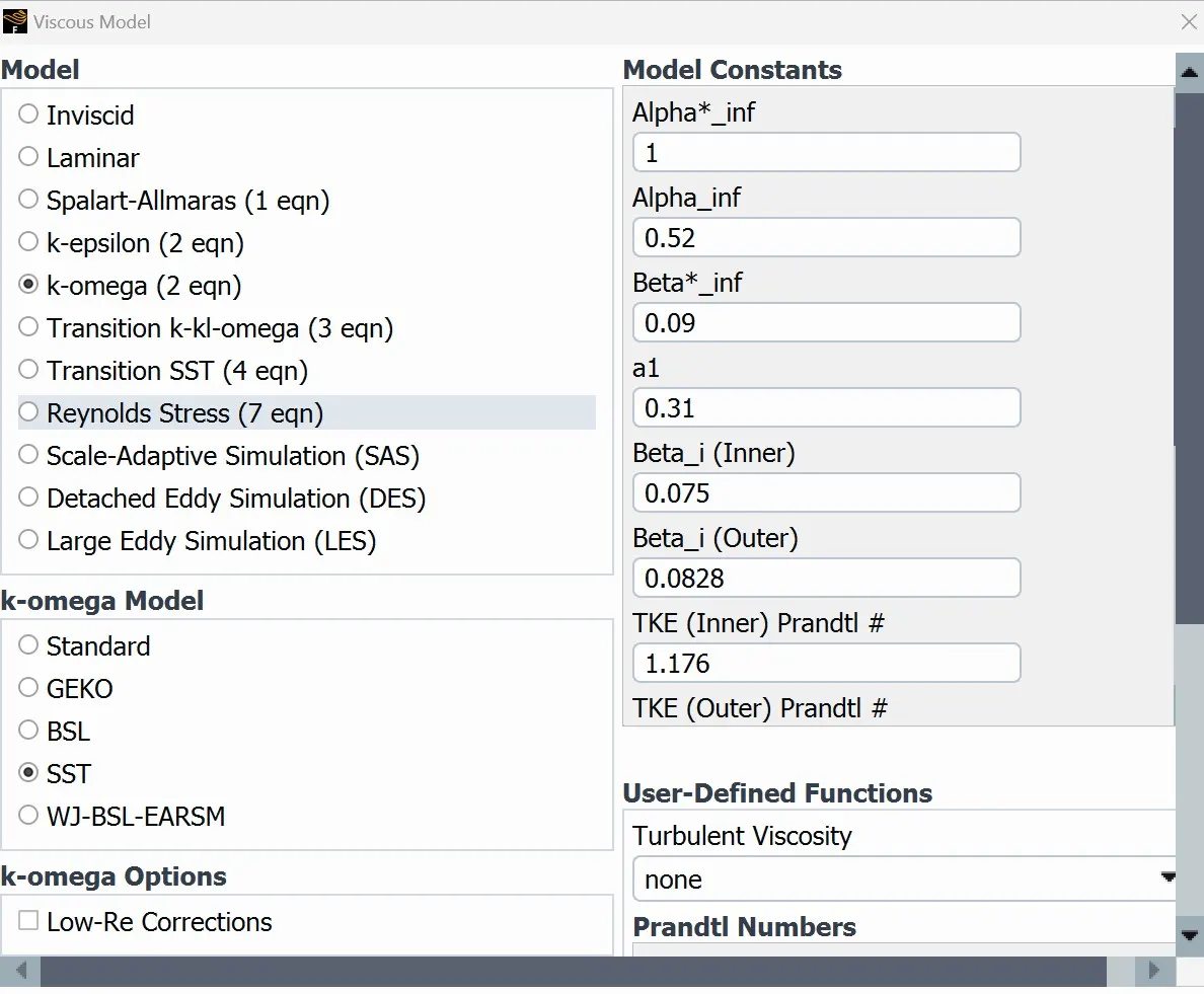
• The K-Omega is used inside the turbulence model.

Result of Residual plots:

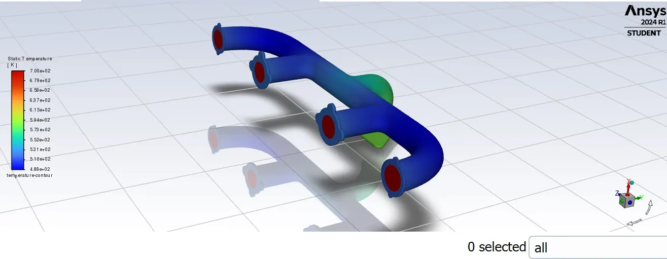
Temperature contour:

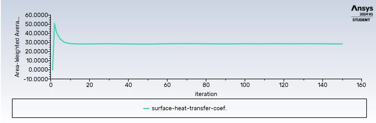
Surface Heat Transfer Coefficient:

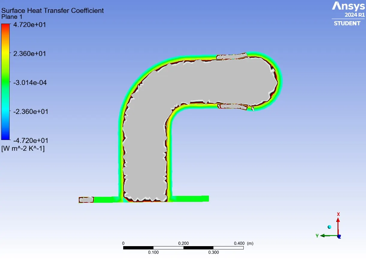
Surface Heat Transfer coefficient on the internal solid surface:

Velocity streamline:

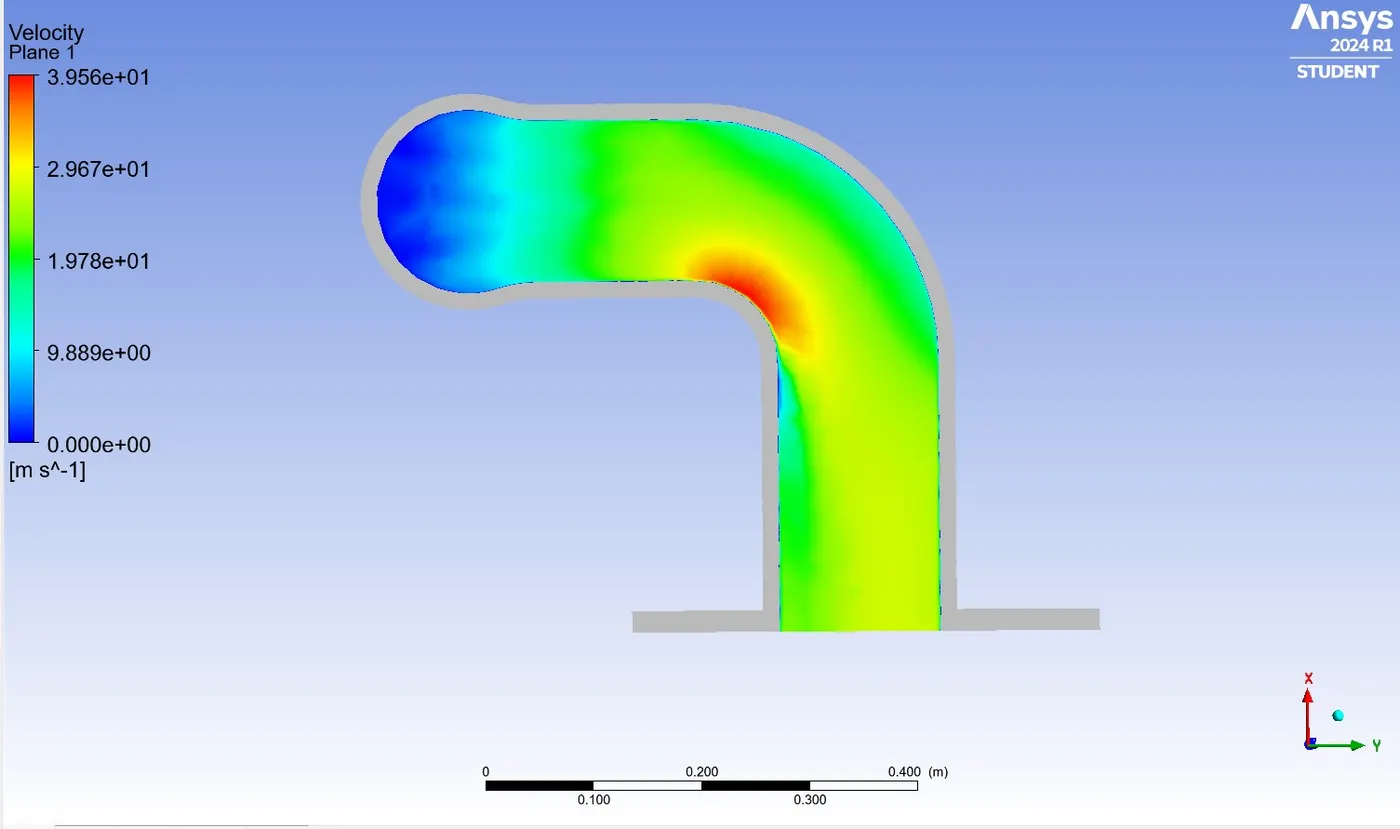
Velocity:

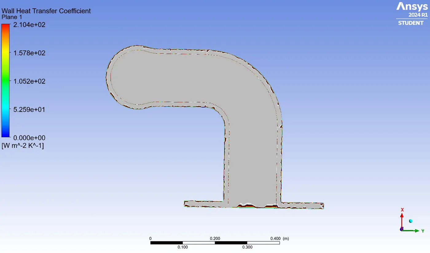
Wall Heat Transfer Coefficient:

Observation:

1. In this model having 4 inlet and one outlet ,when hot air passing through from inlet then the outlet is getting hot as compare to inlet .
2. when hot air is going mixed together in that time velocity going to increase and also temperature.

1. The velocity is higher in outlet region as compare to inlet.
2. We observed from velocity plot , In the bend person having highest velocity region.

Heat Transfer Coefficient at the inner surface:

• The baseline simulation with K-epsilon of inner surface is -21.87 and outer surface is 18.77 . In this simulation, we are getting bed result.
• The refined mesh with K-epsilon of inner surface is 40.76 and outer surface is 34.89 . In this simulation, we are getting not that much good result .
• The refined mesh with K-omega of inner surface is 28.40 and outer surface is 26.66 . In this simulation, we are getting good result .

• The baseline simulation is negative which is bed ,after refinement we are fixed those things.
• We are getting high velocity on the bending person because of that only we are get high temperature at outlet region.

• We are getting more accurate value with the K-Omega.
• The K-omega is recommend for flow near the wall and K-Epsilon for flow away from wall.

• The CHT analysis was explained briefly with its applications and the simulations was performed successfully on the exhaust port.
• The y+ value of 1 was maintained for the refined mesh cases which increased the accuracy of the result.
• The best turbulence model suited for this problem was found to be the K-Omega model.