Week 4 - CHT Analysis on Exhaust port

Aim:

Our objectives are first to give a brief description of why and where a CHT analysis is used. And we need to maintain the y+ value according to the turbulence model and justify the result. Also, Calculate the wall/surface heat transfer coefficient on the internal solid surface & show the velocity & temperature contours in appropriate areas. We need to tell you how you would verify if the HTC prediction from the simulation is right. On what factor does the accuracy of the prediction depend. 

Introduction:

In this challenge, we are going to set up a conjugate heat transfer simulation of an exhaust port. so, now we are going to have a solid model of an exhaust port of an inline four-cylinder engine.

Practical Application:-

Theory:

CHT analysis:

The CHT is conjugate heat transfer. It is the concept of heat transfer involved in both fluid and solid simultaneously. For, solving the CHT problem we use both conduction and convection for the relative phase material. 

Where the CHT analysis is used and why:

Conjugate heat transfer corresponds with the combination of the heat transfer in solids and the heat transfer in fluid. In solid, the conduction is often dominating, and in fluid convection is usually dominating.

For example, The CHT is a heat exchanger by circulates a hot fluid through one section port and it has a colder fluid passed over to another section port. by making use of the solid pipe we can exchange the heat between the two fluids without having them mix.

Maintain the y+ value: 

• Y+ is a non-dimensional distance.
• It is used to determine the first layer thickness distances from the wall which is measured in terms of viscous length. 
• Since there is the transfer of heat in both fluid and solid surfaces. so, we use the k-epsilon turbulence model. To properly capture the fluid parameter at the boundary.  
• by reducing the Y+ value concerning the turbulence model we can easily visualize that more clear temperature and the velocity gradient are observed. 
• so this will give correct results.

K-Epsilon Modeling:

For the RANS-based modeling, we want to model and solve the turbulence velocity. This is an unknown form of the Renold transport equation. for this, we may use the k-epsilon model.

where, 

• K is a turbulent kinetic energy.
• Epsilon is a rate of dissipation of turbulent energy.

Why is the mesh size fine near walls?

The finer mesh helps to capture the wall heat flux and wall shear stresses. These would be required for analyzing quantities (Eg: Coefficient of friction, heat transfer coefficient, etc.) To capture the heat flux and shear stress a fine mesh enough would be needed to resolve the boundary condition. Hence the mesh resolution is needed in the boundary layer.

What is the Reynolds number?

It is the ratio of initial force and viscous force. so, the idea is here to understand the impact of flow trying to move in a domain and its inherent frictional force trying to stop the flow from flowing in the domain. It is a dimensionless number.

Re = Rho*V*L/mu 

Where,

• ρ - Density of the fluid 
• V - velocity of the fluid
• L - characteristics of the length 
• μ - viscosity of the fluid

It helps to segregate the flow into:

Laminar (Re<2300 - Internal flow, Re<1*105 - External flow)

Turbulent (Re<4000 - Internal flow, Re>5*105 - External flow)

What is the Nusselt number?

It is the ratio of convection heat transfer and conduction heat transfer within a fluid region. Nusselt number denotes the increases in heat transfer through a fluid layer caused by convection. When the fluid is motionless then conduction will be the dominant mode of heat transfer so the (Nu = 1) and when the fluid is a bulk motion then convection will be the higher. It is a dimensionless number.

Nu = hL/K

Where,

• h - heat transfer coefficient of the fluid
• L - characteristics of the length 
• K - Thermal conductivity of the fluid

What is the Prandtl number?

It is the ratio of the momentum diffusivity to thermal diffusivity. It compares between the velocity boundary layer thickness and the thermal boundary layer thickness. The Prandtl number for Gases is about 1. For the water is in order of 10. for liquid meta is 0.01 and for heavy oil is 105. It is a dimensionless number that measures the efficiency of transport by momentum diffusivity to thermal diffusion.

Pr = nu/alpha

Where,

• ν - momentum diffusivity
• α - Thermal diffusivity

Analytical calculation for verifying and validating HTC:

To calculate the HTC for turbulent flow in a tube, since the fluid that is flowing through the exhaust port is air, so we need to know the properties of air. So, to get the properties of air Go to setup -> Go to physics -> Go to Material (create/edit) -> Select the material type and fluid materials is fluid and air an then click "OK".

This is for case 2,

 

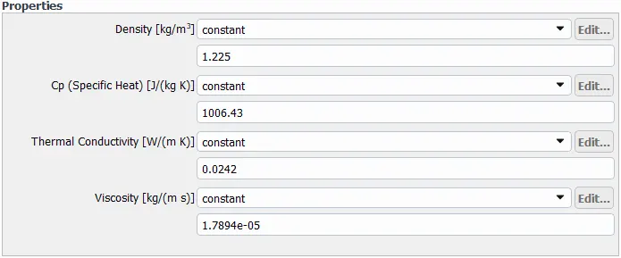
• Density, ρ = 1.225 [kg/m²]
• Specific heat, C_p= 1006.43 [j/(kg k)]
• Thermal conductivity, κ = 0.0242 [W(m.k)]
• dynamic viscosity, μ = 1.7894x10⁵[kg/(m.s)]

we know the Reynolds number,

Re = ρ.V.D/μ

Where,

• Velocity V = 5 m/s
• Diameter D = 166.11 mm

Now substitute the value in the above equation, 

we get, Re = 56,853.

We know the Prandtl number,

Pr = ν/α

Pr = v/(κ / ρ.C_p) 

Pr = ρ.v.(C_p / κ)

Pr = μ. (C_p / κ)

Where,

• μ = ρ.v

Now substitute the value in the above equation, 

we get, Pr = 7.441*10^11

Hence, the Re = 56853 which is greater than 10000, we used the Dittus Boielter equation for the fluid being heated.

The Dittus Boielter equation is used to calculate the surface HTC for fluids in turbulent flow inside a clean round pipe.

According to the Dittus Boielter equation, Nu = 0.023*Re(0.8)*Pr(0.4)

Nu = 0.023.(56,853*0.8).((7.441*10^11)*0.4)

Nu = 7.7839*10^14

We know the Nusselt number,

We get, Nu = h(D/k)

Where,

• Diameter, D = 166.11 mm
• Thermal conductivity, κ = 0.0242 [W(m.k)]

h = Nu.(k/D)

HTC (h) = (7.7839*10^14.(166.11/0.0242))

h = 5.199*10^19

Pre-processing & Solving Setting:-

  

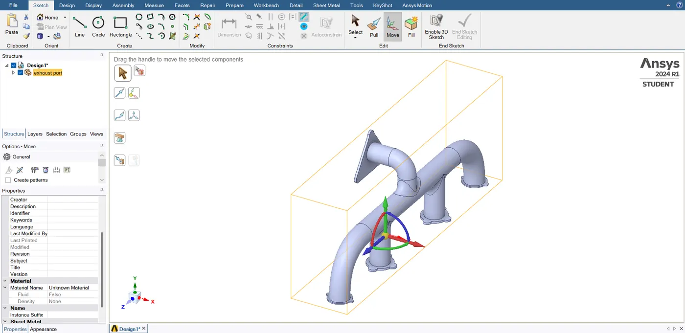
• Now we are going to set up a conjugate heat transfer simulation of an exhaust port. now we are going to have a solid model of an exhaust port of an inline four-cylinder engine. And then we are going to be, modeling both the fluid through it and also the solid heat transfer. and this is called conjugate heat transfer(CHT). so, first, open the workbench and then add the fluent, and then open the geomentry in SpaceClaim. Now, first thing change the unit into "meter" and then import the geomentry from the folder. just drag and drop it here. 
• Now the geomentry is loaded. so, that's our exhaust port this is a made-up geomentry. but it contains all the features that an actual exhaust port would have right. so, our objective is basically to simulate the flow through it and as the flow is going through the manifold. how it is going to exchange the heat with the solids. we want to simulate that process. 

  

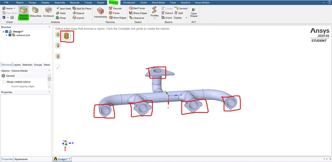
• so to do that we are going to assume initially that the flow that coming through the exhaust which is basically all these four inlet we are going to assume that the fluids are really hot and it basically that the fluid is really hot. It basically that's going to heat the solid pipe from inside.
• All right and on the external surface we are assuming that you know there is a particular heat, transfer coefficient. all right so, in the real-world scenario, the engine is air-cooled meaning it is exposed to air. and air is the particular heat transfer coefficient that is the air near the exhaust port has a particular heat transfer coefficient that would be provided as the input that typically depends upon the Reynolds number of the external air.
• in this case we are going to specify that there is a particular valve of a transfer coefficient and that's going to determine the heat transfer rate. so, now if I take a closer look at the geomentry you can see that it has the solid part. so the first step that I need to do is to extract the fluid volume.
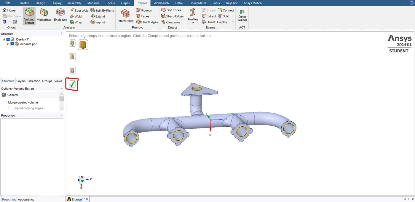
• To do that go to the prepare section and select the "volume extract". and then if I go to the edge selection tool. I can select all four inlets and one outlet. and then click on "ok".

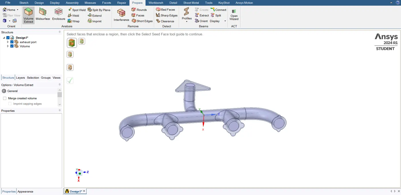
• so, now you can see that our fluid volume has also appeared. so in the design, I'm going to call this "fluid volume". and rename that to "solid volume". so, now close this "geomentry" and then open the "mesh" GUI. 

  

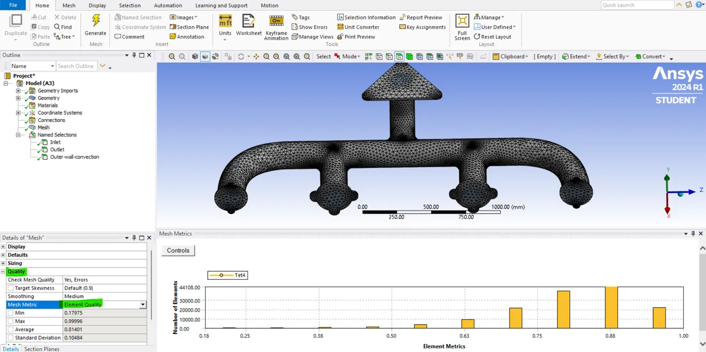
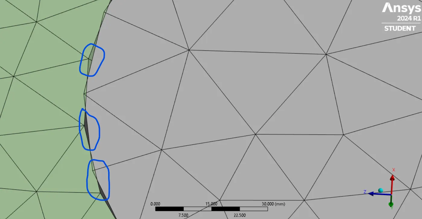
• After opening this meshing interface let's first generate the basic mesh to get a feel for what's actually happening. so, here you can see the problem is that we have a kind of solid that the fluid volume and solid volumes are separated parts right inside the meshing interface and hence we have something called a non-conformal mesh, meaning ideally you know this particular vertex should be connected to this vertex right. this particular phase should be connected to this particular phase. then only the heat is going to get transferred smoothly. but here it's not happening like that. so, we need to fix this.
•  The non-conformal meshes what we have here. so, for example, here you can see that there is actually a physical gap between those two bodies. we can actually fix this a little bit, but then for, conjugate terms of simulatons. we want this to overlap perfectly. so the two vertex are connected to each other.

   

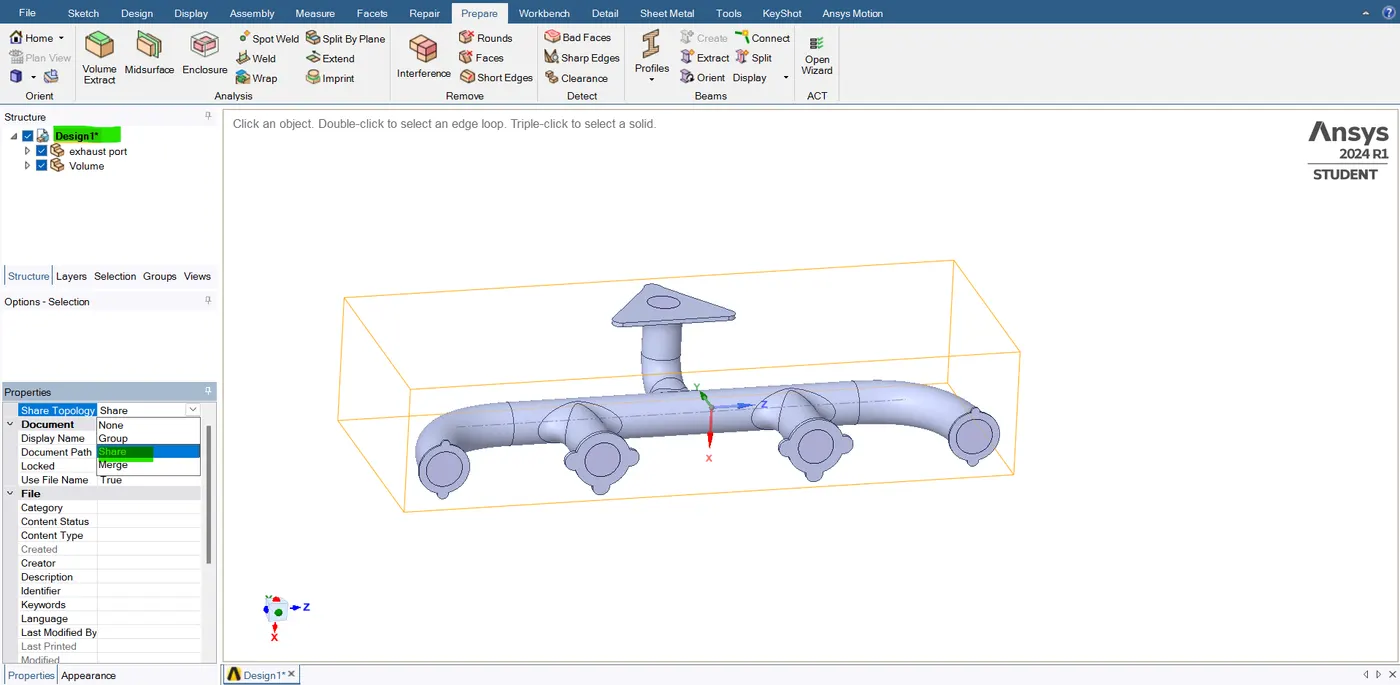
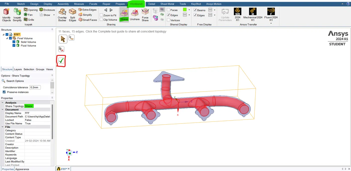
• Now to do that what we need to do is we need to do something called "share topology". so, let's go back to the geomentry. and close this meshing. 
• Before opening the geomentry just reset the meshing and open the"geomentry" GUI. so, now the properties enable the shared topology into "share". so, whenever the shared topology is enabled the two interfaces are shared and that will actually help us to create the mesh correctly.

  

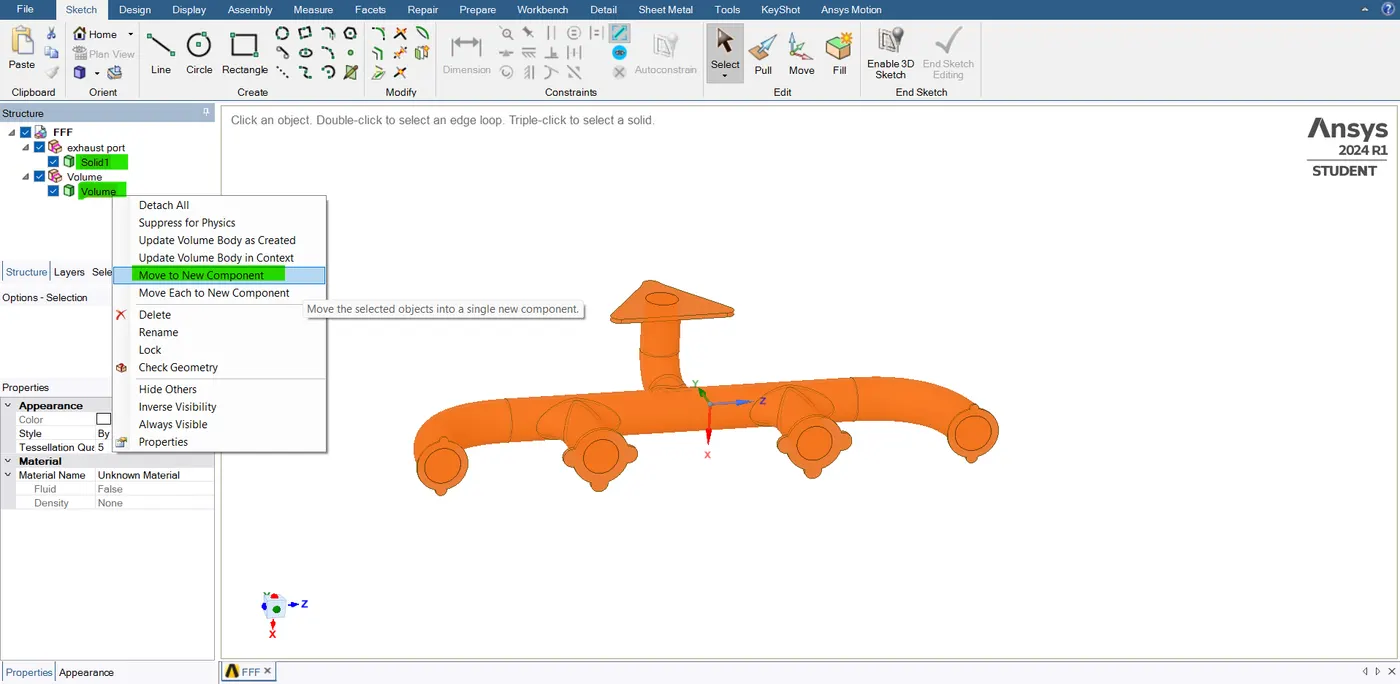
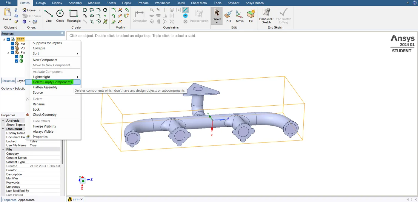
• Before we do the share there is an important step that we need to follow and that step is you need to first take your two volumes. right click on these two volumes and then move it to a new component and then name it as a "final geomentry". and now right on"FFF" and then select "delete empty components". After that enable that share topology to do that first go to the workbench and enable the "share" hit the share button.

  

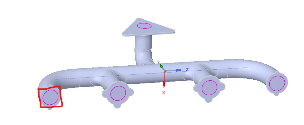
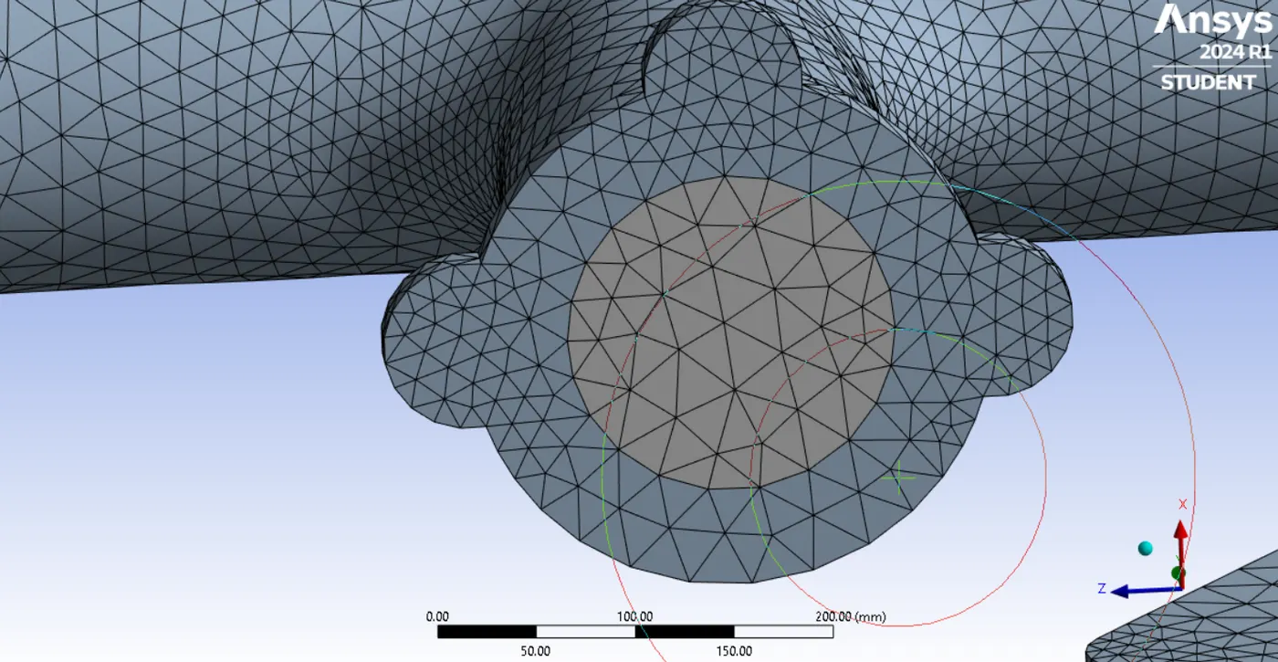
• The share topology is a very important step. if we don't do this step and if we directly go to the meshing interface then the mesh will definitely fail. so, that we need to take care of creating the interface between your solid block and fluid block. after doing this we can able to see the pink circles are created here it basically tells you things are being shared. now go back to the mesh interface if you look at the mesh it's perfectly created. and this is exactly how you need to be making the meshing for a conjugate heat transfer simulation.

 

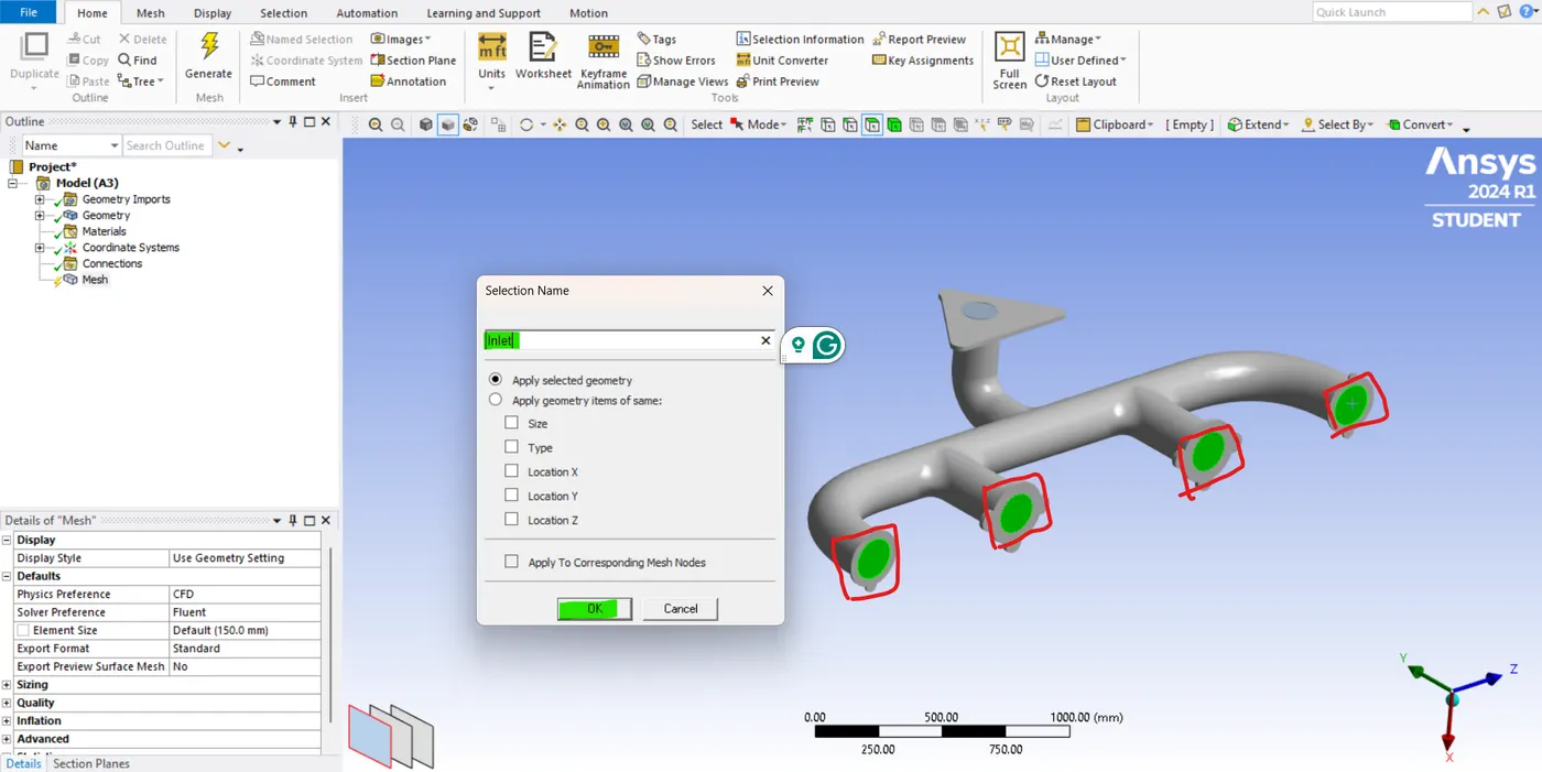
• So, now right-click the mesh and then clearly generate data why because. we are not selecting any name surfaces that we want to do. just select the "face select tool" and then select the 4 inlets and click "N" in Typepad and name it "inlets". 

 

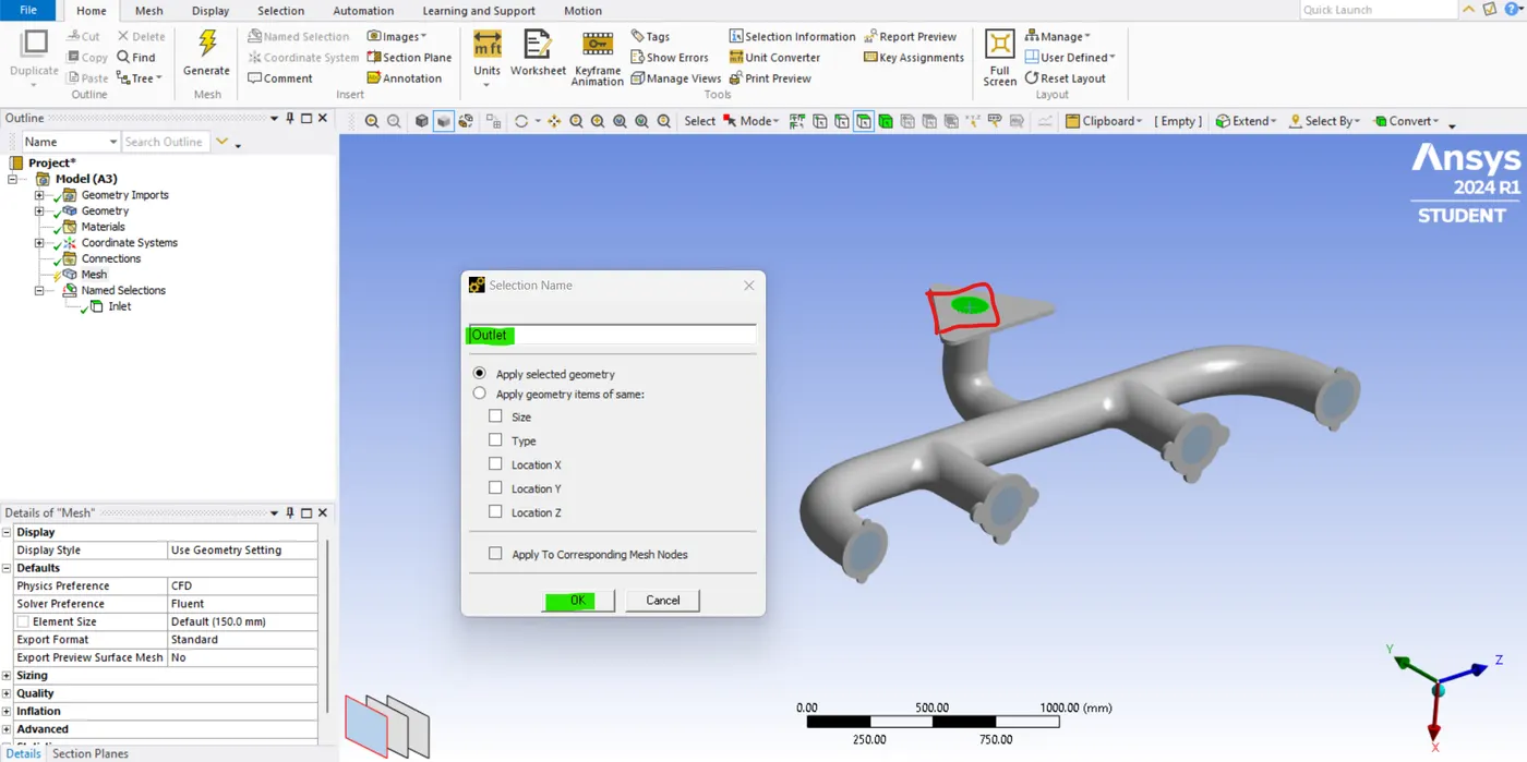
• similarly, select the other opposite outlet face and name it an "outlet".

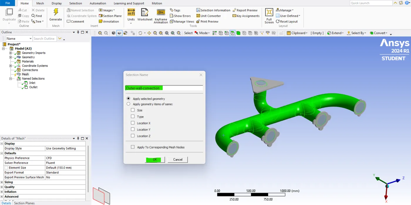
• similarly, select the outer surface and name it an "outer wall convection".

   

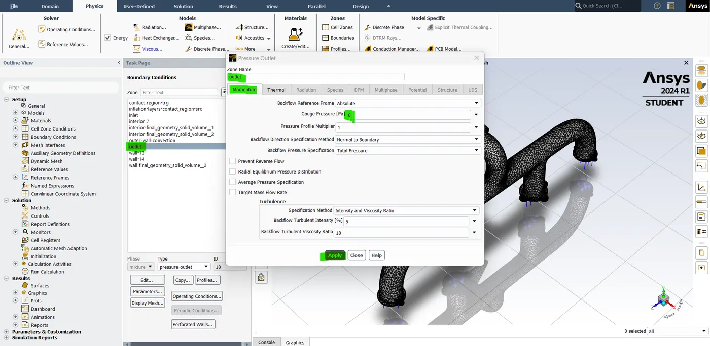
• Now you can see that there are additional walls. those "walls" into a setup interface. and these walls basically have adiabatic boundary conditions which are exactly what we want. 
• now click on quality and select metric mesh. now you can see that these are the cells that have poor quality. so, we can fix this problem by adding mesh refinement.
• so, looks like our inflation mesh did get created. so let's take a look at the total cell count. we are about a quarter million cells. so, still, we can able to do refinement. so, now I'm going to add a few more cells in the solid component.
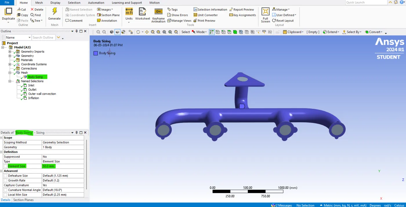
• so, to do that right right-click on the mesh insert and add "sizing". I'm going to select this body and apply. and the sizing element size is set to 50 mm. so, let's take a look at the mesh and how it works out. and if you take a look at the total cell count. it's pretty much something. so, we need to decrease the mesh to 12 mm. Now it looks more accurate let's close this mesh GUI. After that update the mesh.

  

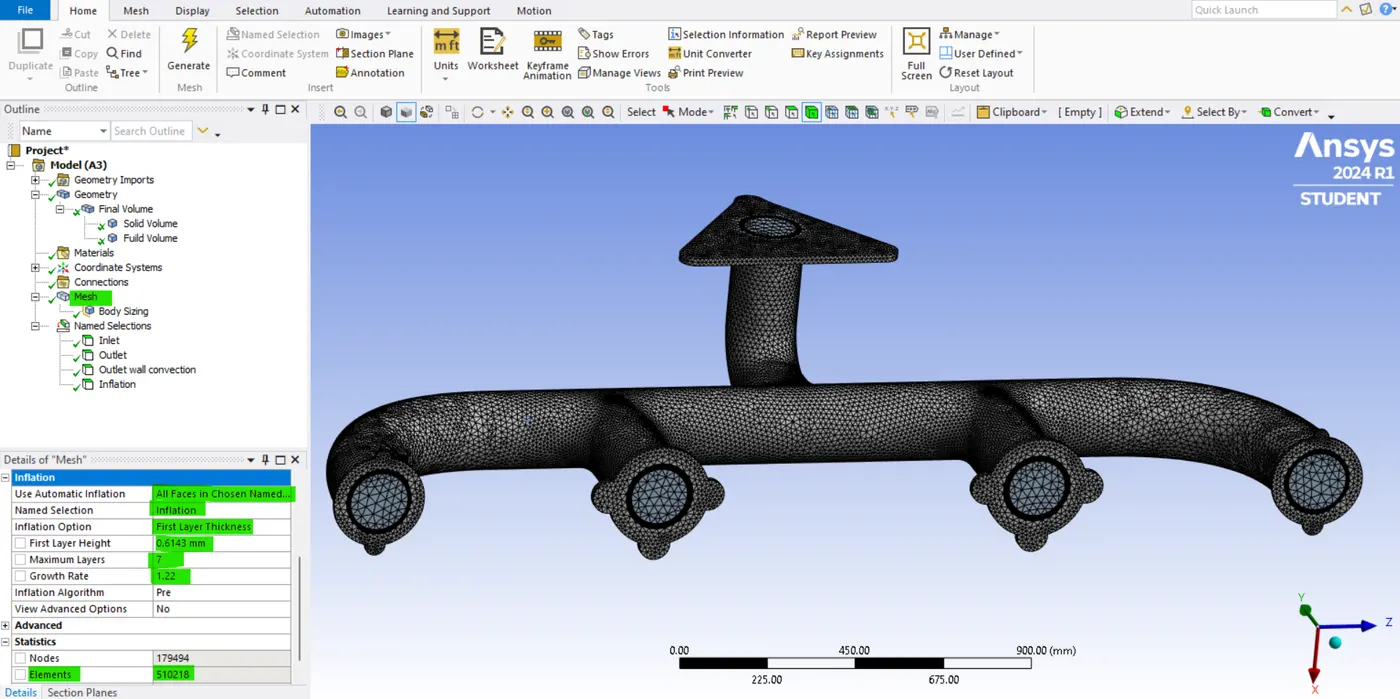
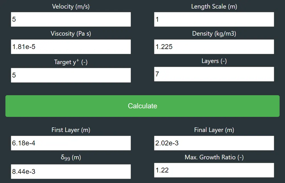
• So, now I'm going to refine the mesh. so, open the mesh interface and after that, we can add an inflation layer for the internal volume to make things better. so, to calculate the Y+ first layer thickness we need to use the y+ calculator.
• now to add the inflation layer go to inflation -> select All faces to chosen named selection -> select the "inflation" in the named section -> select the First layer thickness and the first layer height is 6143 mm -> maximum layer is 7 -> growth rate is 1.22.

  

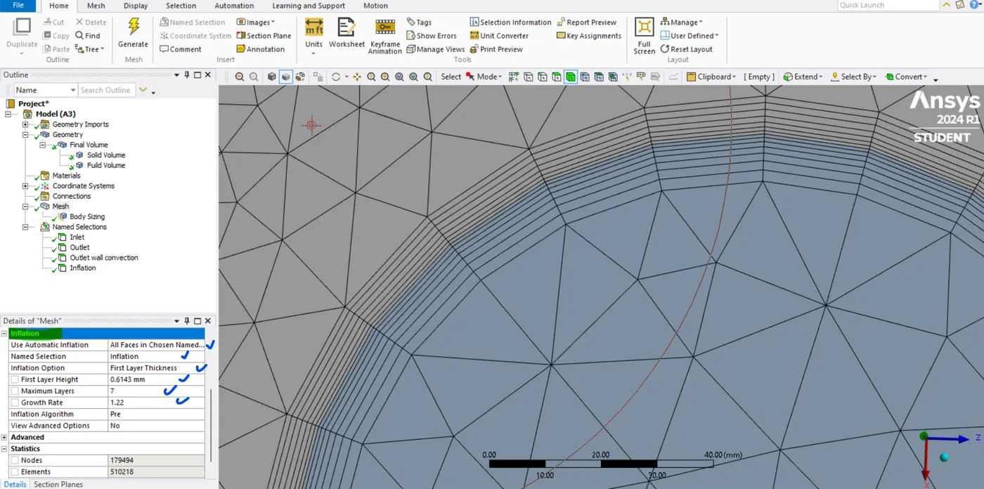
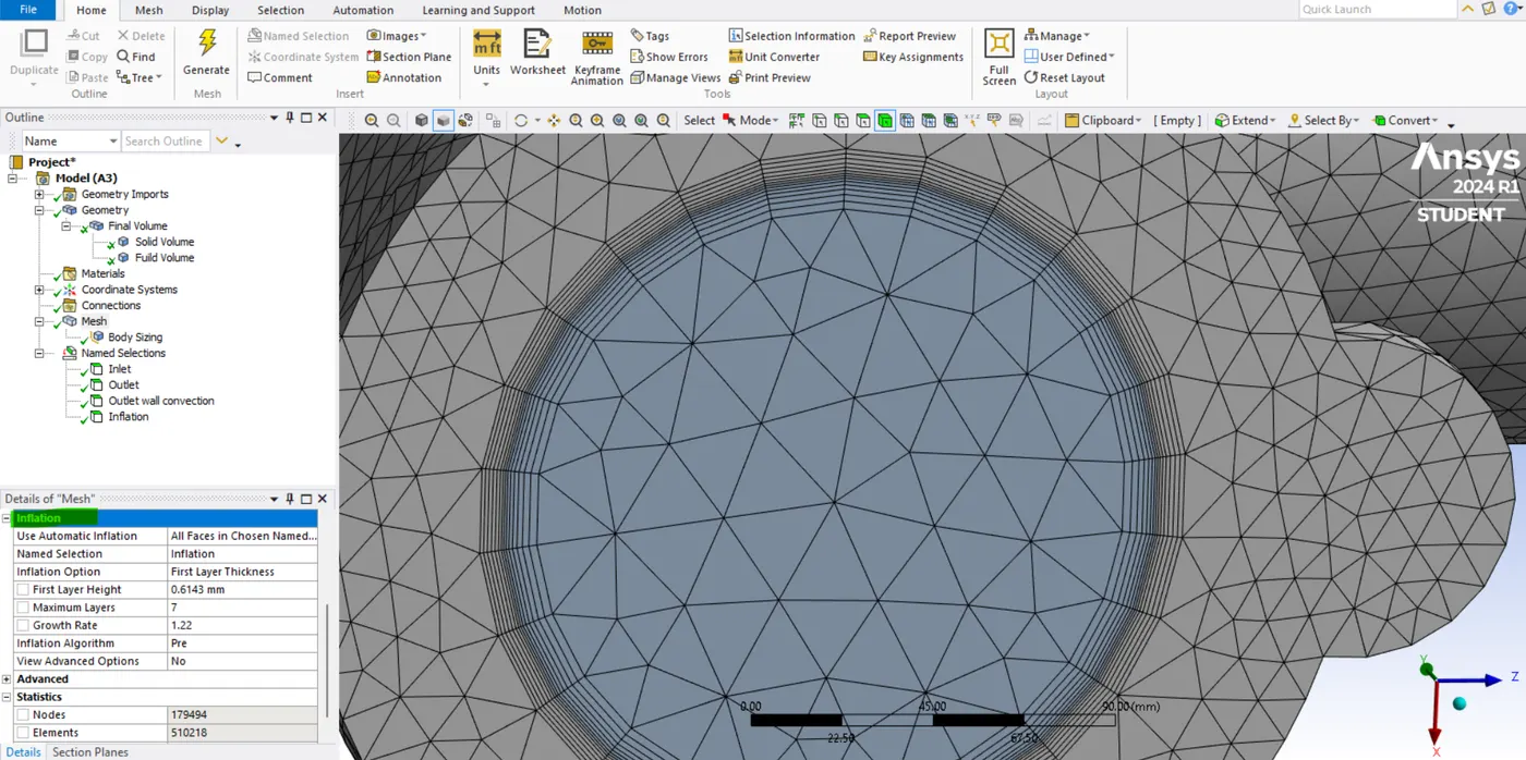
• Now you can see the inflation layers have been created perfectly so, now the surface heat transfer coefficient is captured accurately in the wall region. After that now, update the mesh so that we can move to the setup part. 

Solving & Modelling Approach:-

  

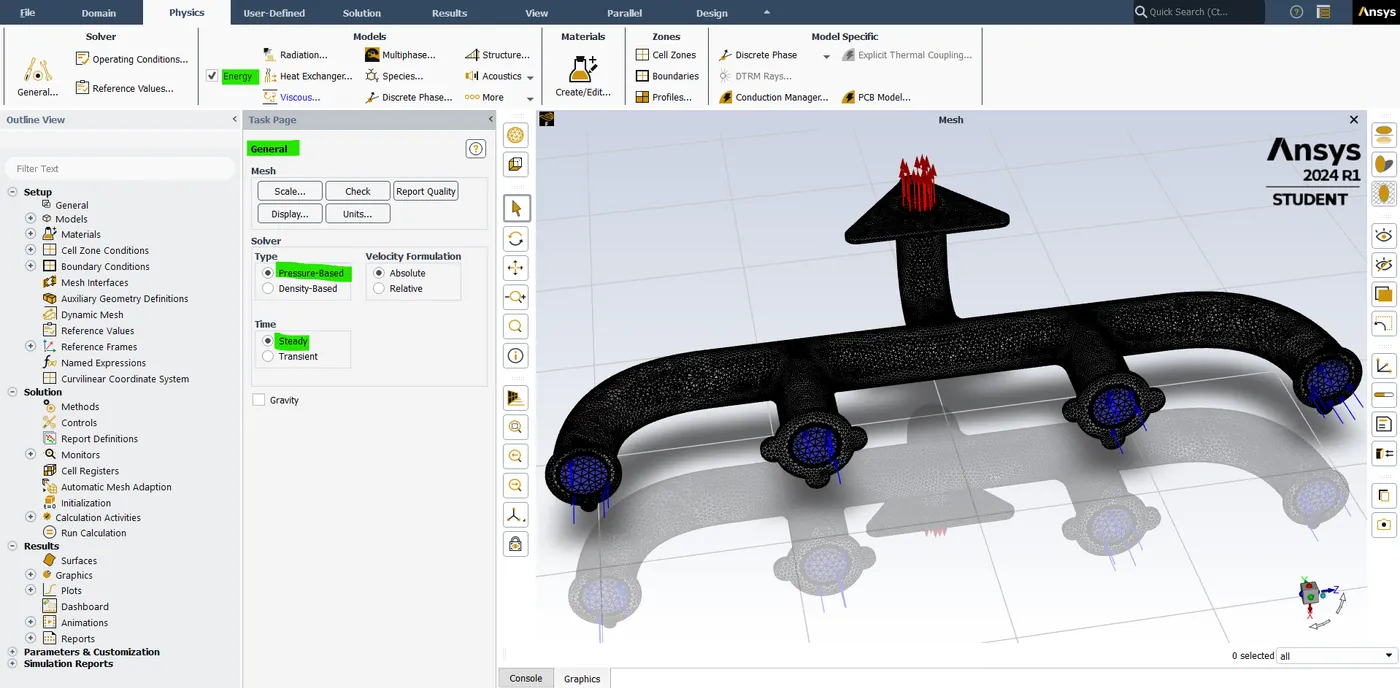
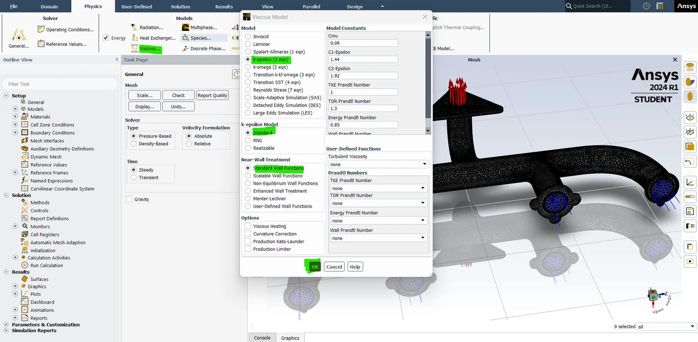
• For both baseline mesh and refined mesh the three-dimensional equations are solved using a pressure-based solver. for modeling the turbulences the standard k-epsilon model is employed.
• now close the meshing interface and then open the setup GUI. now you can see that the geometry of the inlet and outlet have automatically been colored. so, that's a very nice visual representation that is consistent.
• now, we are going to use a "pressure-based solver" in this case and we are going use "steady-state analysis". so, this is fine so, let's go to setting up physics. we are going to be solving the energy equation now, for the viscous model. we are going to be using the "k-epsilon" turbulence model. and then go to the physics section and click materials. so, in that the "fluid is air" and the "solid is aluminum" so, that's fine.

   

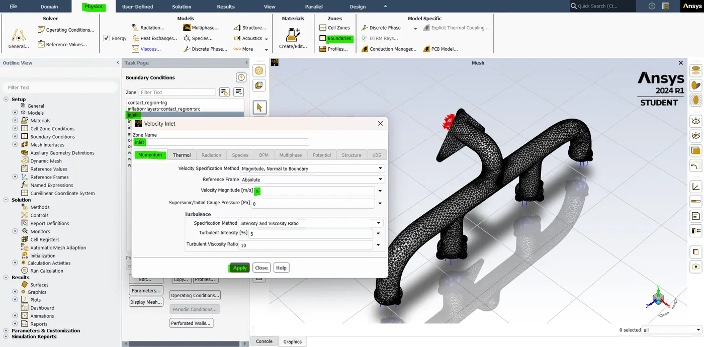
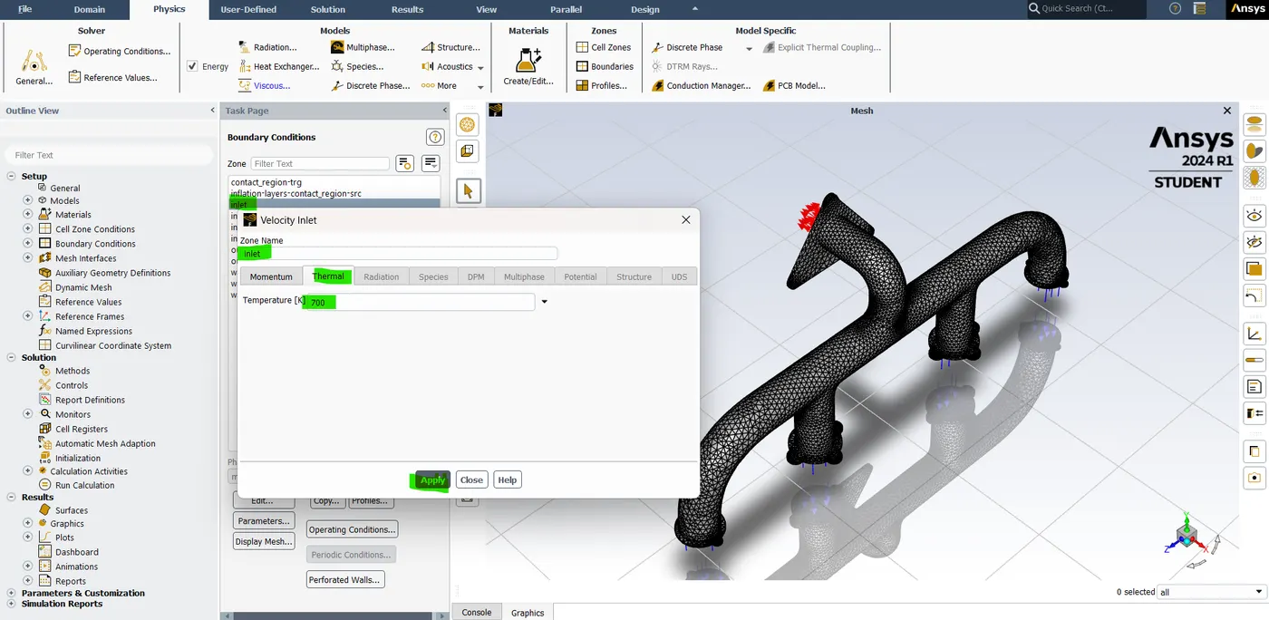
• Now go to boundary condition and click on "inlets the velocity is 5 m/s" and the thermal is "700 k". hit "ok". now you can see that there are a lot of other components. so if you don't understand what these components are then go to setting up domain click on display and then go to setting up. domain click on display. and then we can see every component. but now let's close this domain.

  

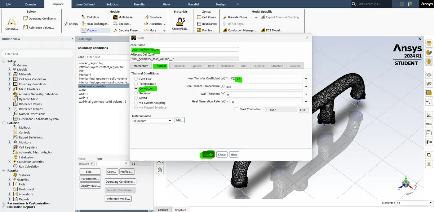
• So now let's click on "outer wall-convection" and in that select "convection" because the boundary condition is going to be the convection heat transfer coefficient. and I'm going to say that it's 20 Watts per meter sq kelvin. this value is based on some kind of experimental data and some research papers there you know what is the heat transfer coefficient of the air around the exhaust port. 

  

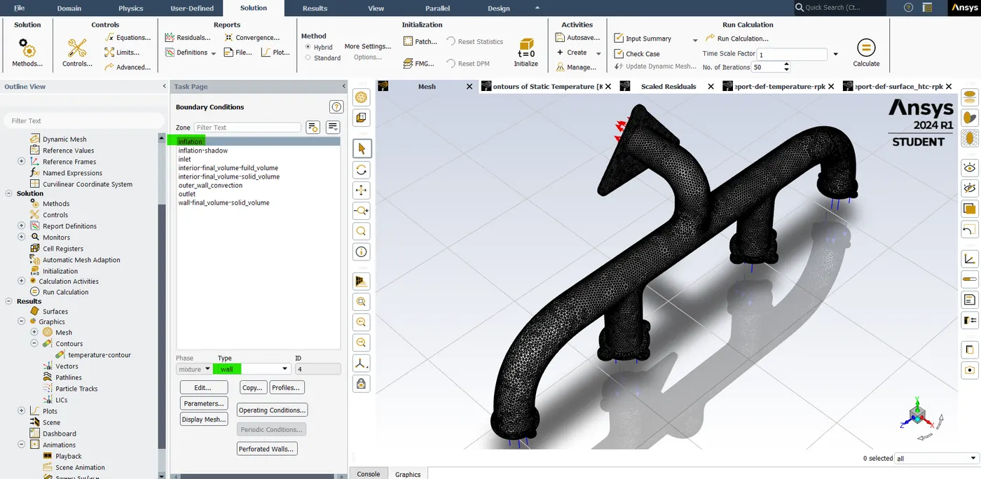
• For inflation we need to select the type "wall". why because then only in the result part we can create an inflation mesh on the plan correctly. if we do not change this into the wall then the inflation mesh will be a course and the heat won't be able to be captured in the wall boundary properly. 

   

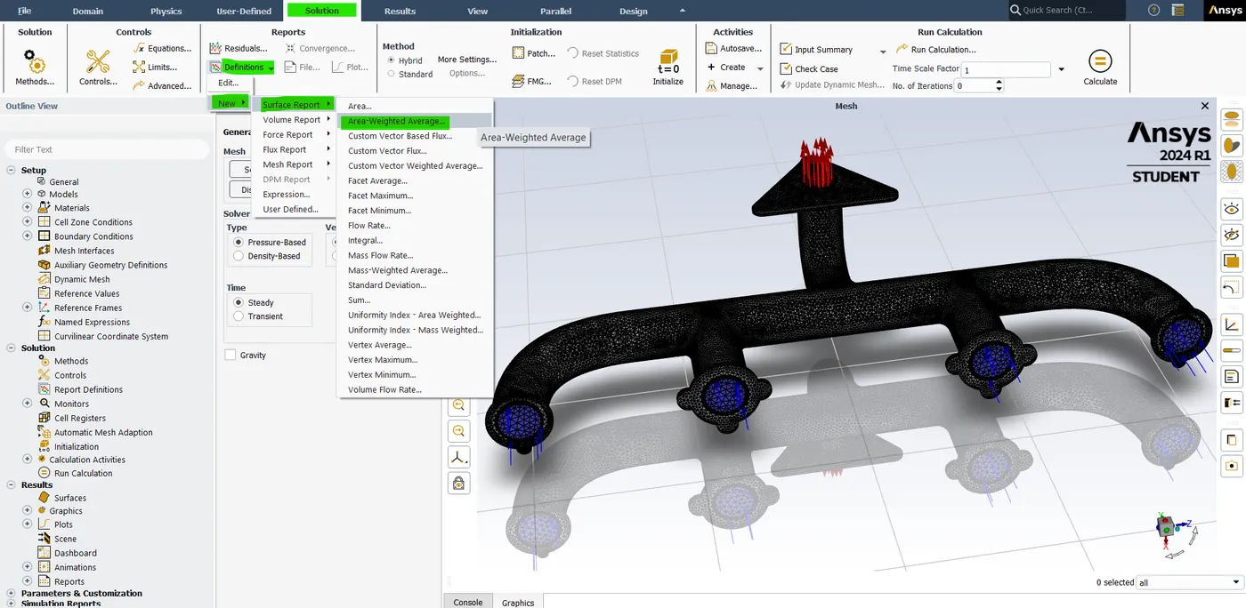
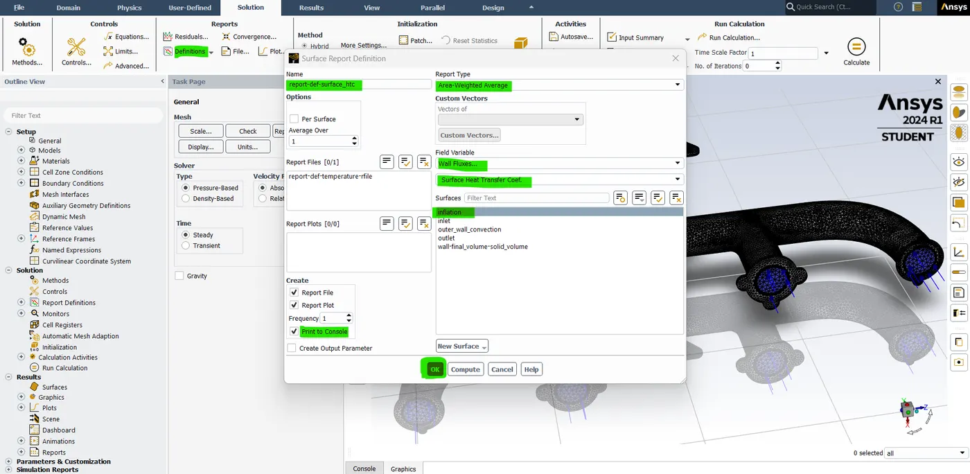
• Now we need to create the definition plot for the Surface heat transfer velocity on the "inflation" under the wall flux in the Area-weighted average and select the print to the console.

 

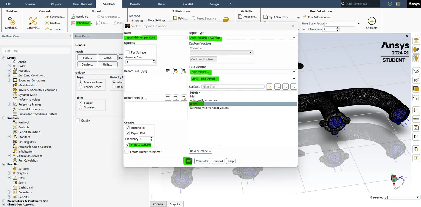
• Now add the definition plot for the temperature on the "outlet" under static temperature in the Area-weighed average and select the print to the console. 

  

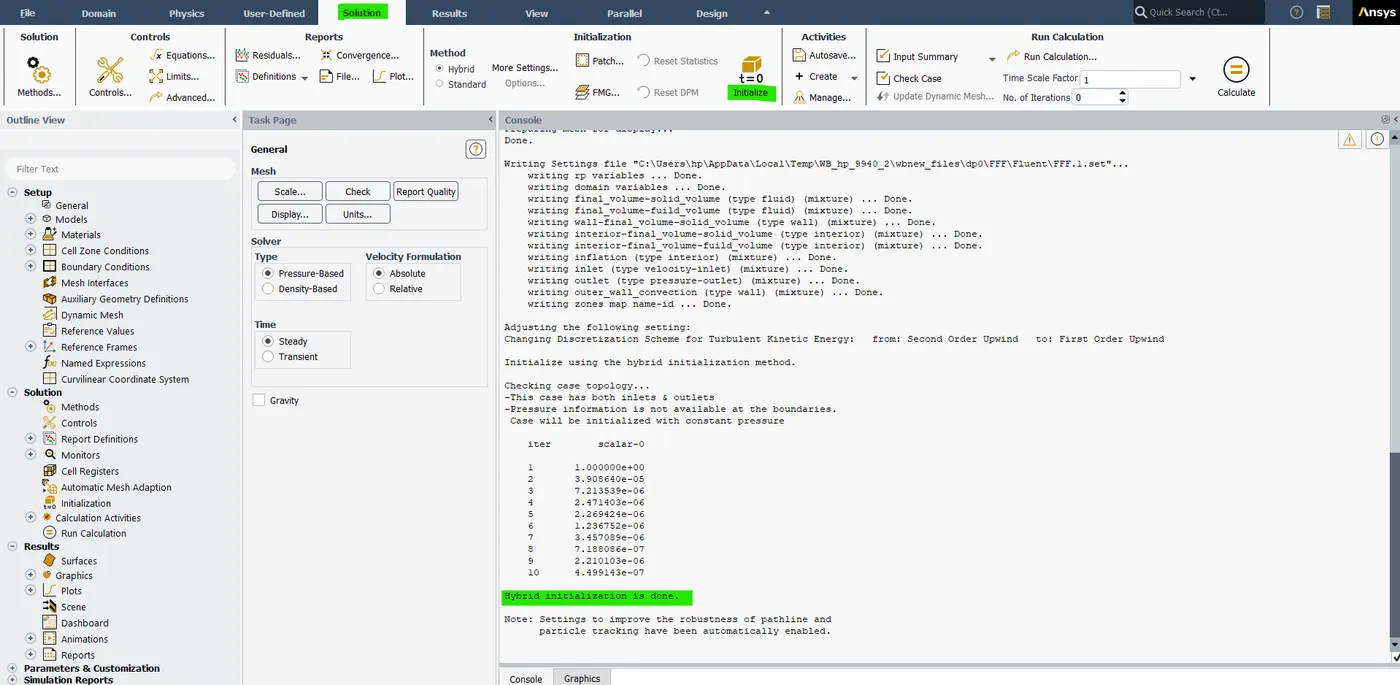
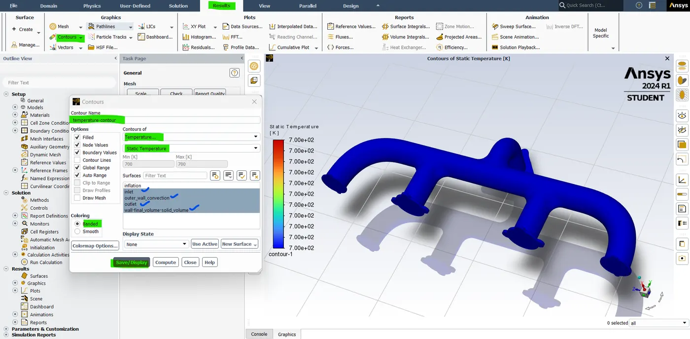
• so, the heat transfer coefficient is 20 watts per meter square kelvin. and there are many other boundary conditions. so, we are just going to ignore them. so, now go to the "solving" section and then I'm going to initialize the "hybrid initialization" The initialization is done. after that go to "post processing" and click "contoure" new. now name the contour "temperature" select the temperature in the contour type and select surface as "inlet" "outlet wall convection" and "outlet" and the "final boundary" and now click on "save/display". so, that looks good. so, we can see here the initial temperature is set to 700 Kelvin. that's fine. 

  

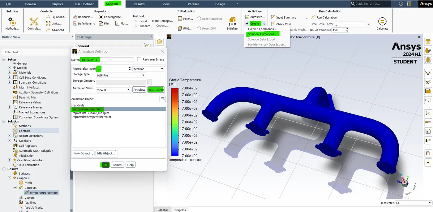
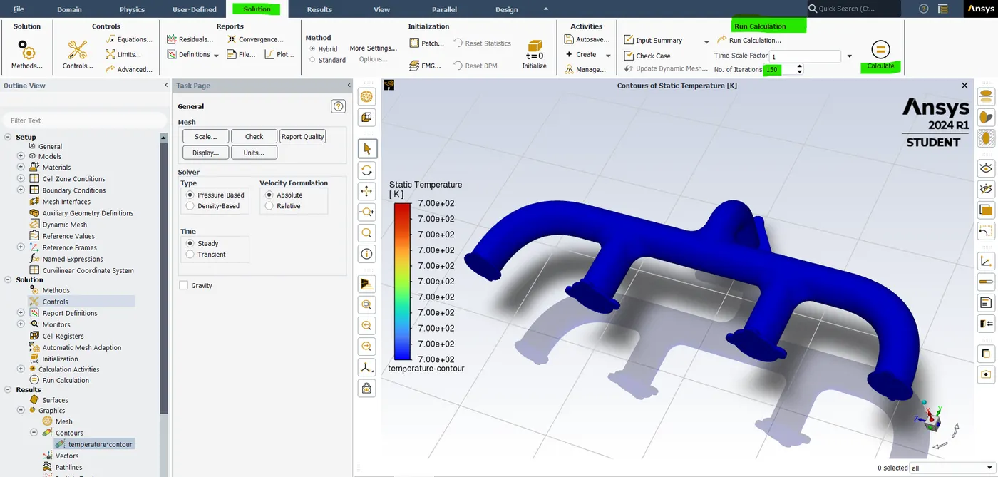
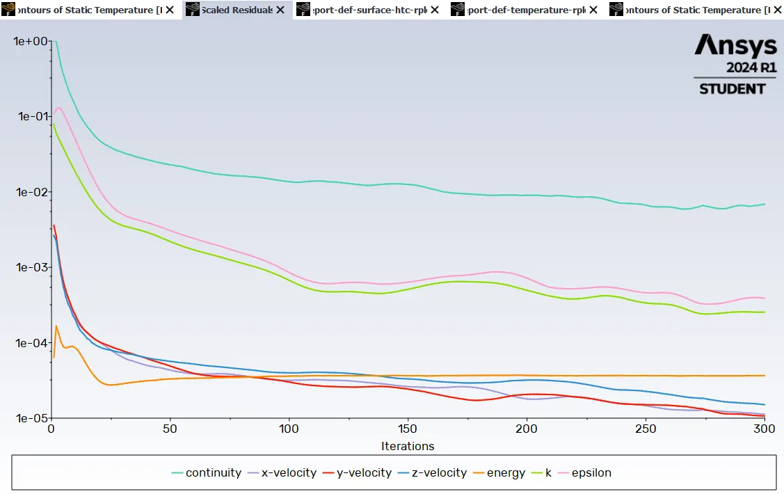
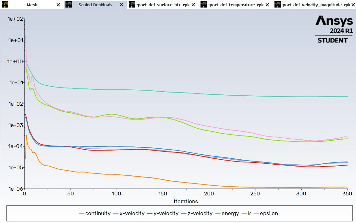
• Now go to "solving" and hit "calculate" 150 iterations. before that, we need to create some "solution Animation". And I'm going to look at the temperature contour and set the required view and click on preview and hit"ok". And hit the "calculate". And see how the simulation is running. so, now the simulation is completed. if you look at our residuals you see that's continuously dropping. but it looks like our static temperature contours are converged. if I go to "animation" playback. the temperature is developing and it's changing very slowly. so, it looks like the solution is converged around. 120 interactions.

  

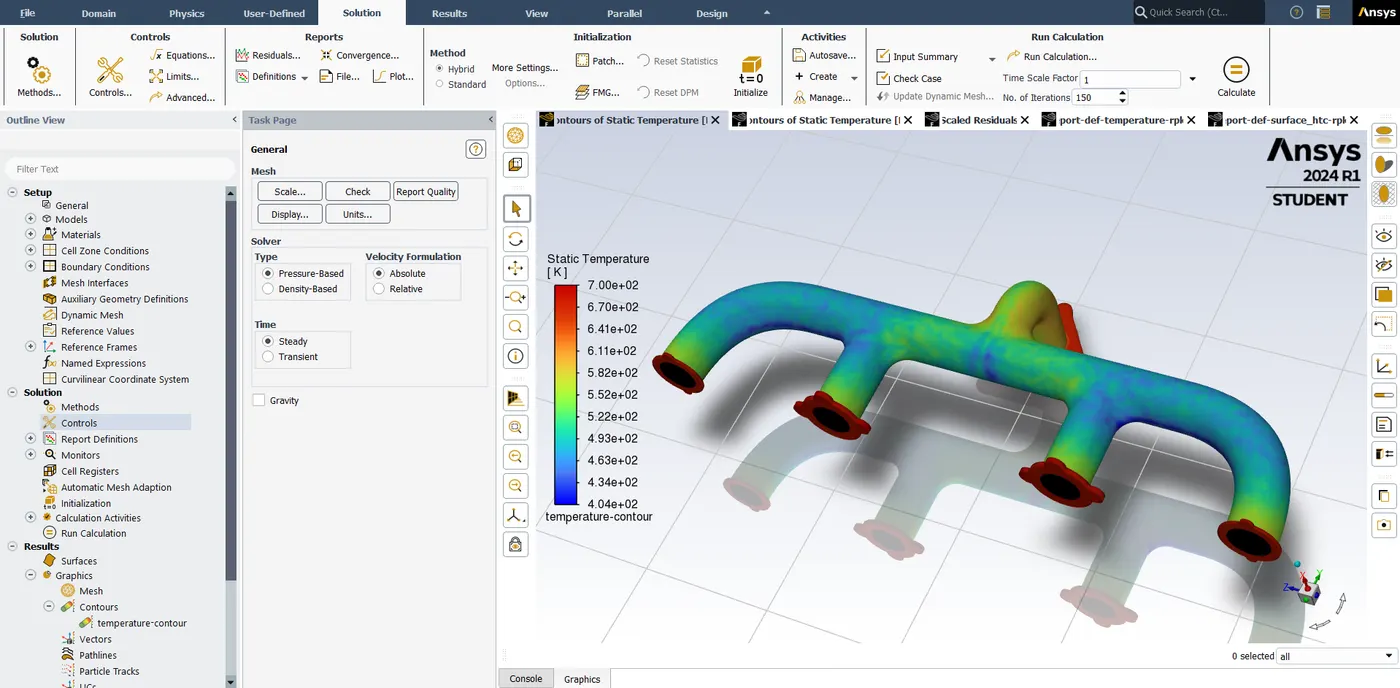
• so, you can see that the heat is getting diffused here but then that's basically it after some time it stops right after 90 or 95 iterations with slight improvement. we can call it a "steady state temperature distribution". Now the solution has converged and we need to compute some value through the simulations. 

      

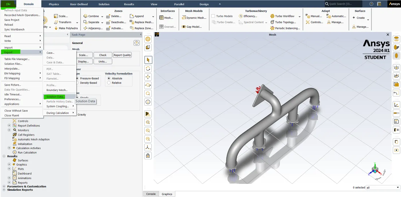
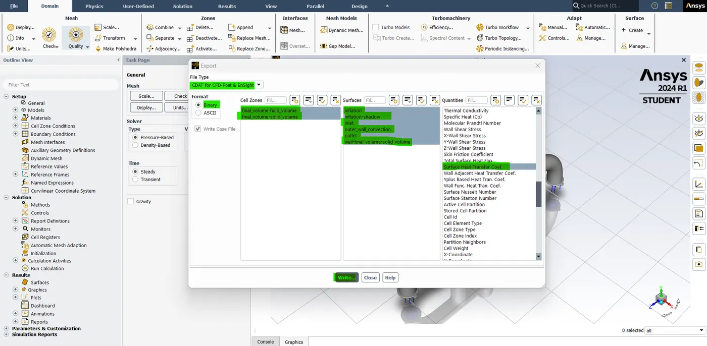
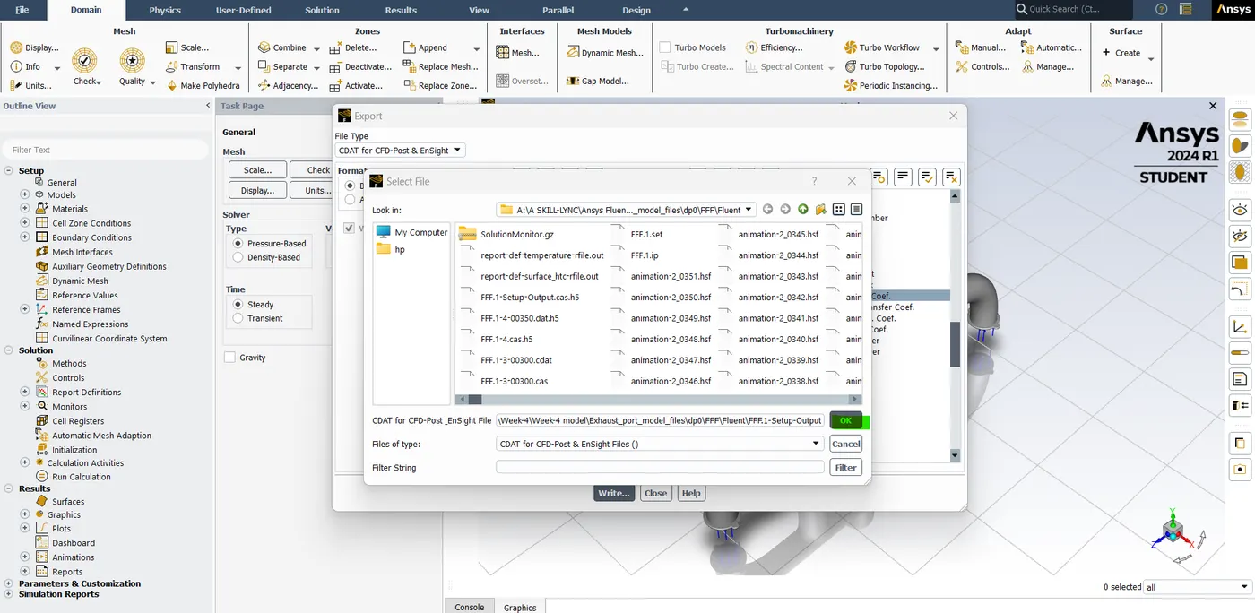
• Now before moving to the result part we need to export the solution data, so then only we can able to visualize the surface heat transfer coefficient. To do that go to the file -> click Export solution data -> now the new window is pop-up in that select the file type is CDAT for CFD-Post. Select the format "Binary" and the cell zone "fluid volume and solid volume" and then select the surface is completely and the select the quantities as a "surface heat transfer coefficient" and then hit on "write". now we need to select the file locations and then click "ok". so, now close the setup.

Post-processing:- 

  

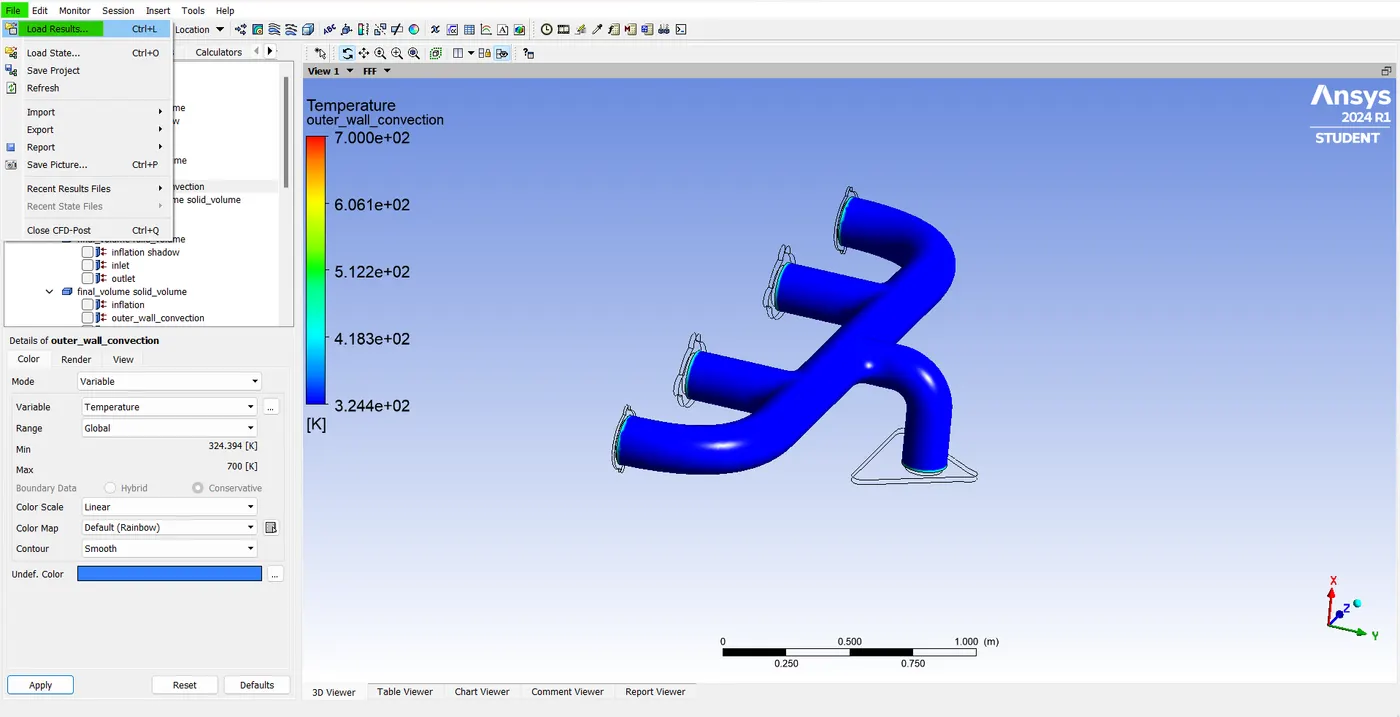
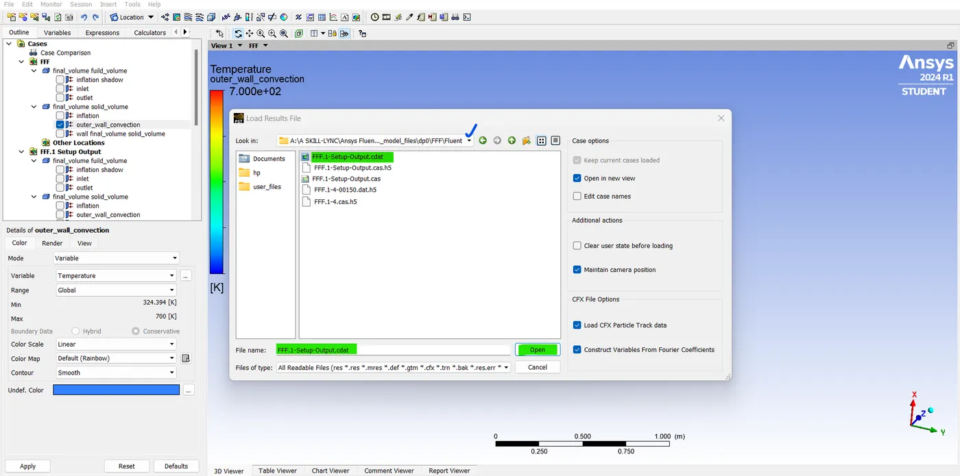
• Now close the setup and open the result "post-process" So, the first thing that I'm going to do is Load the Results meaning import the solution data from the setup section. To do that first go to files -> load result -> select the CDAT location and then hit "open". 

  

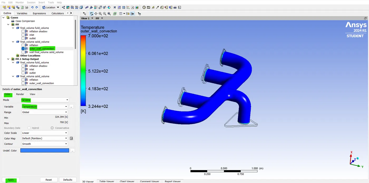
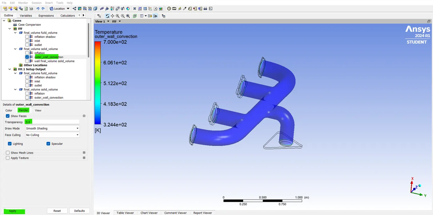
• So, after this, the first thing that I'm going to do is in the solid volume I'm just going to enable the "outer wall convection". and then I'm going to color it as the "temperature" and then go to render to make it a bit more transparent.

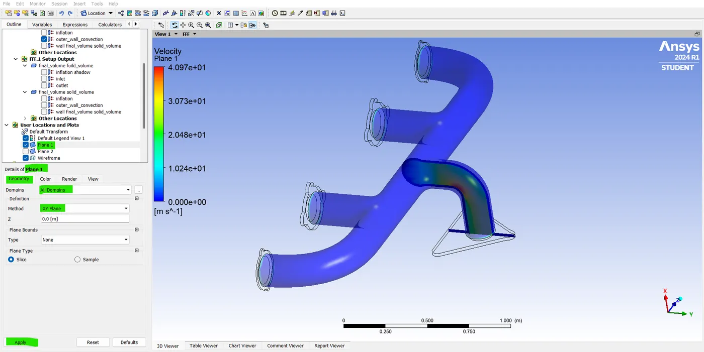
• so, now we can also insert the plane, and let's just call it as a plane-1 and click "apply". and also we need to color this plane so, I'm going to select the variable as a velocity and click "apply".

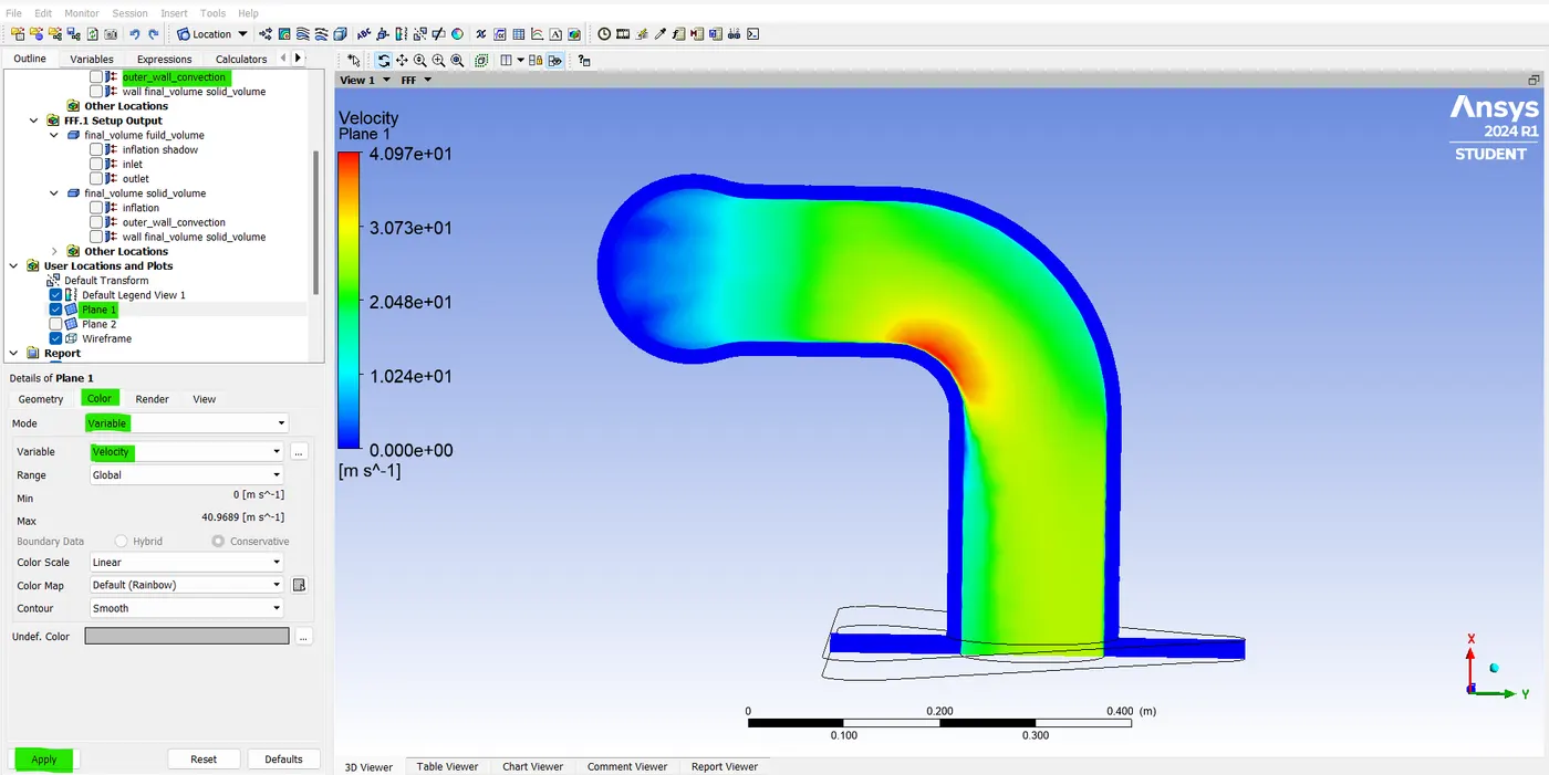
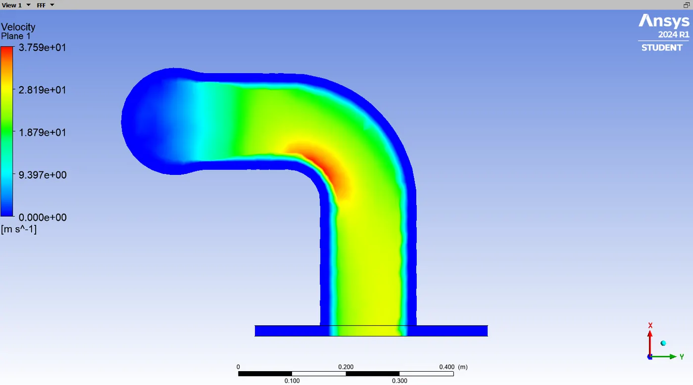
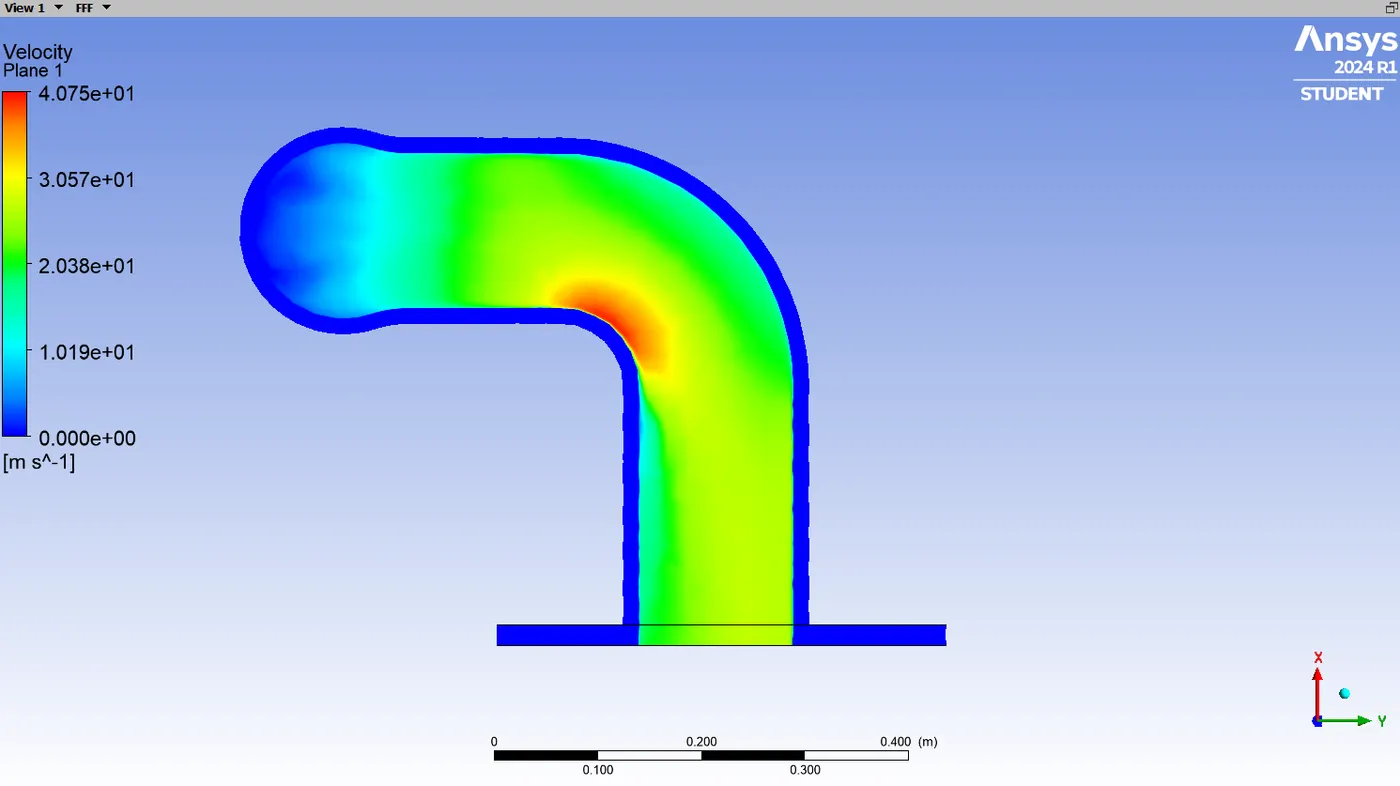
• If I actually colored it by velocity information. now you can see where the higher velocity is and that is where the heat transfer coefficient is higher. and that's why the location where maximum heat transfer is taking place and since the fluid is hot. so, it will have the maximum amount of heat transfer from the fluid to the solid which results in a higher temperature of the solid at that particular location. 

  

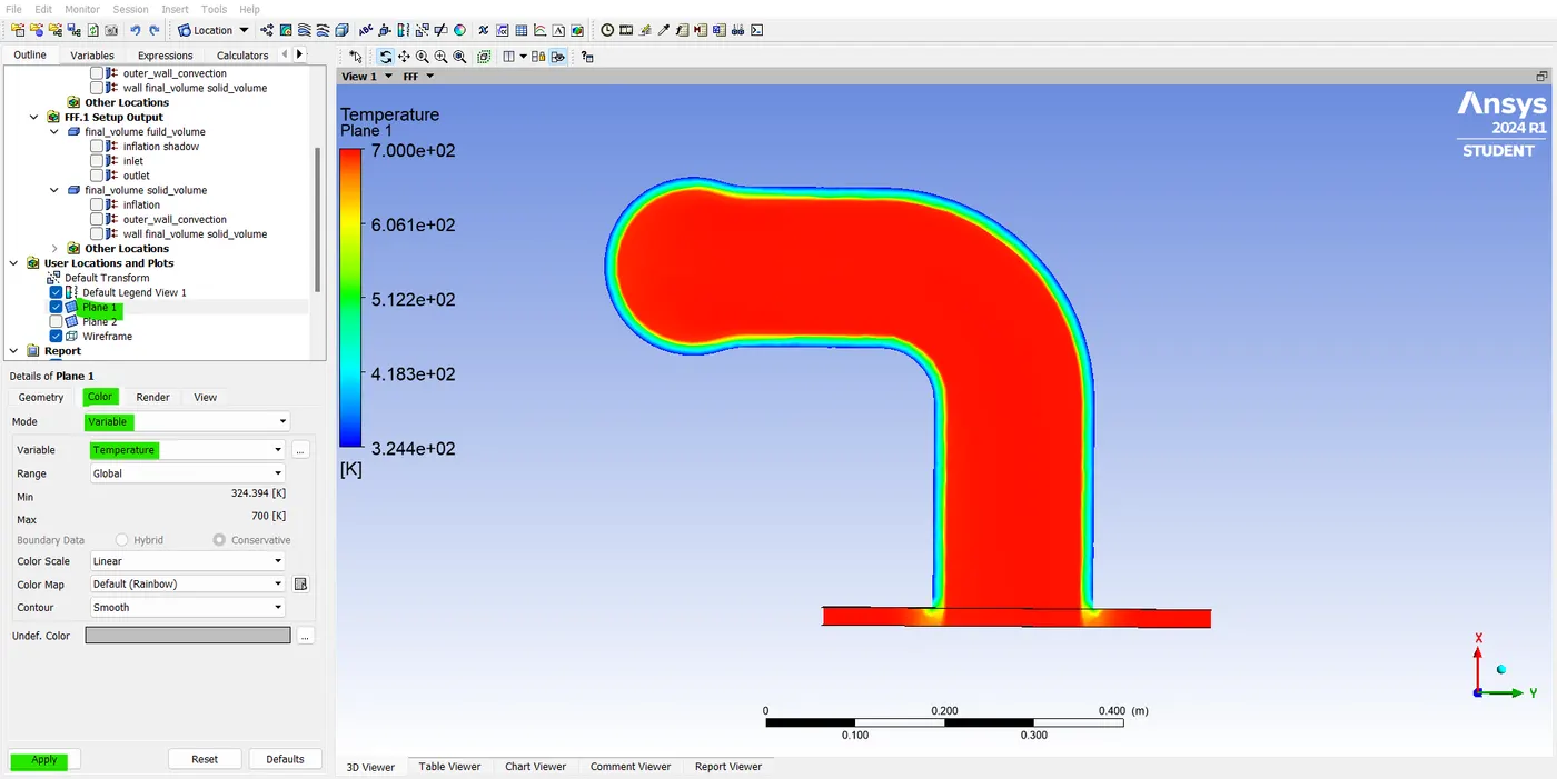
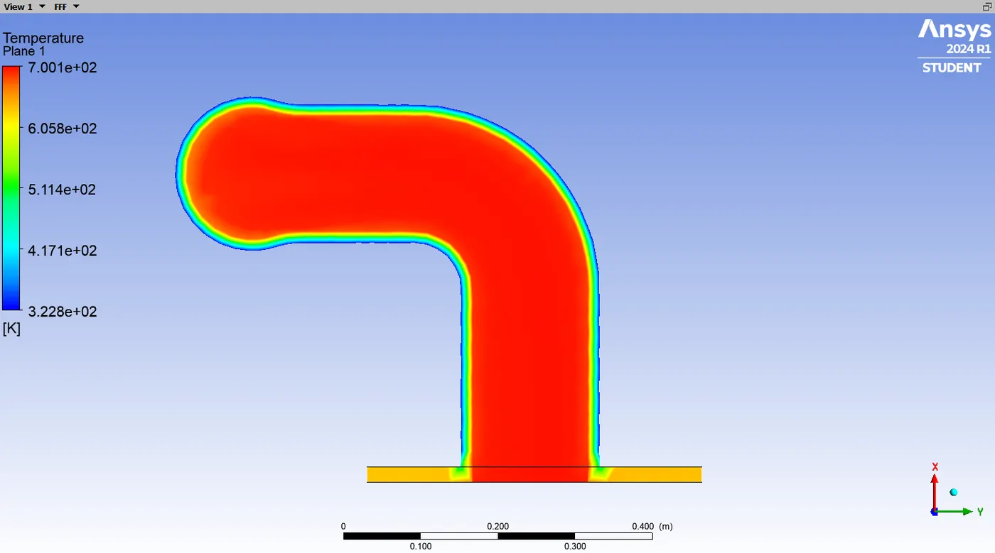
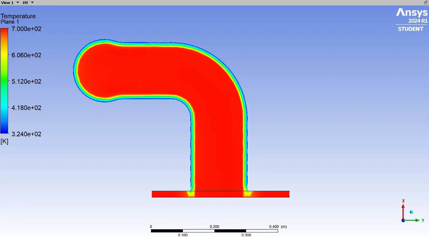
• if I look at the temperature in plane 1 you can see the maximum temperature occurs in all areas except the wall surface of the plane. in that wall surface region, there is minimum temperature is maintained why because the boundary layer less than 0 layer there are low temperatures. so, the temperature is started only in the first layer and it continuously increases.

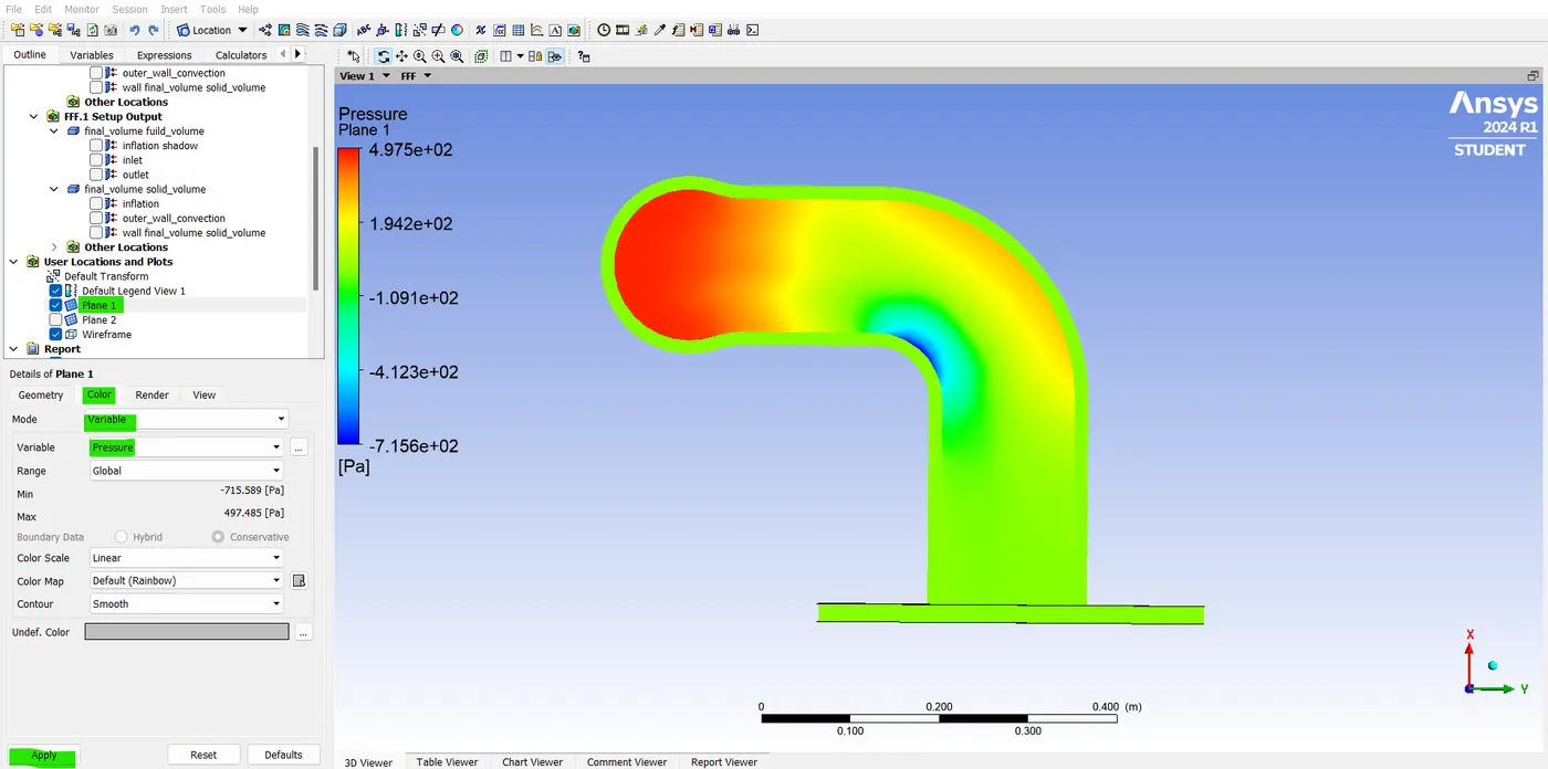
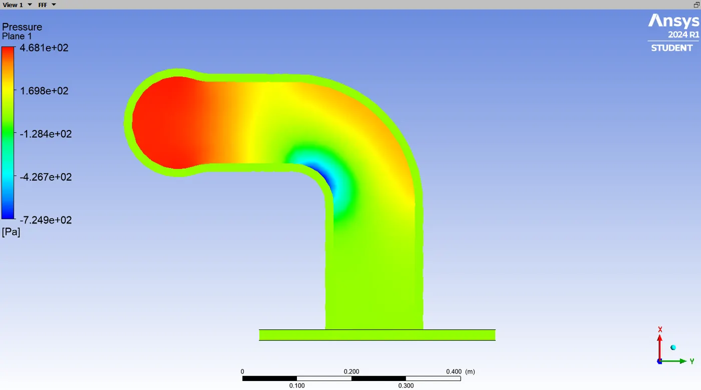
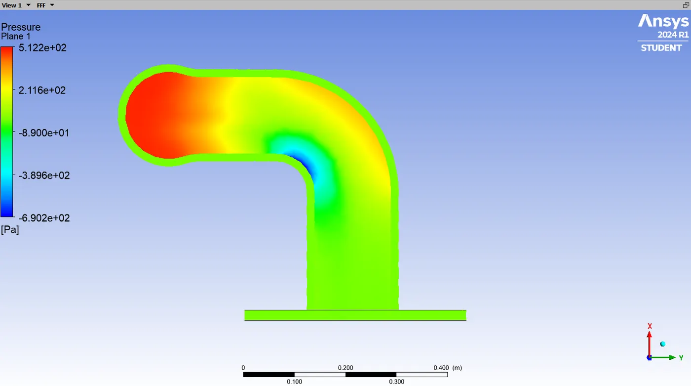
• you can see the maximum pressure take place at the initial place of the plane-1. 

  

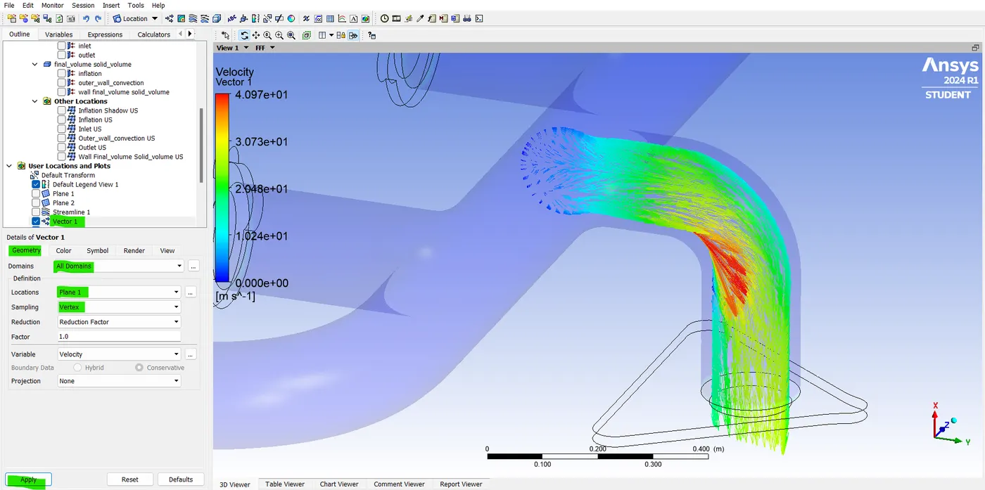
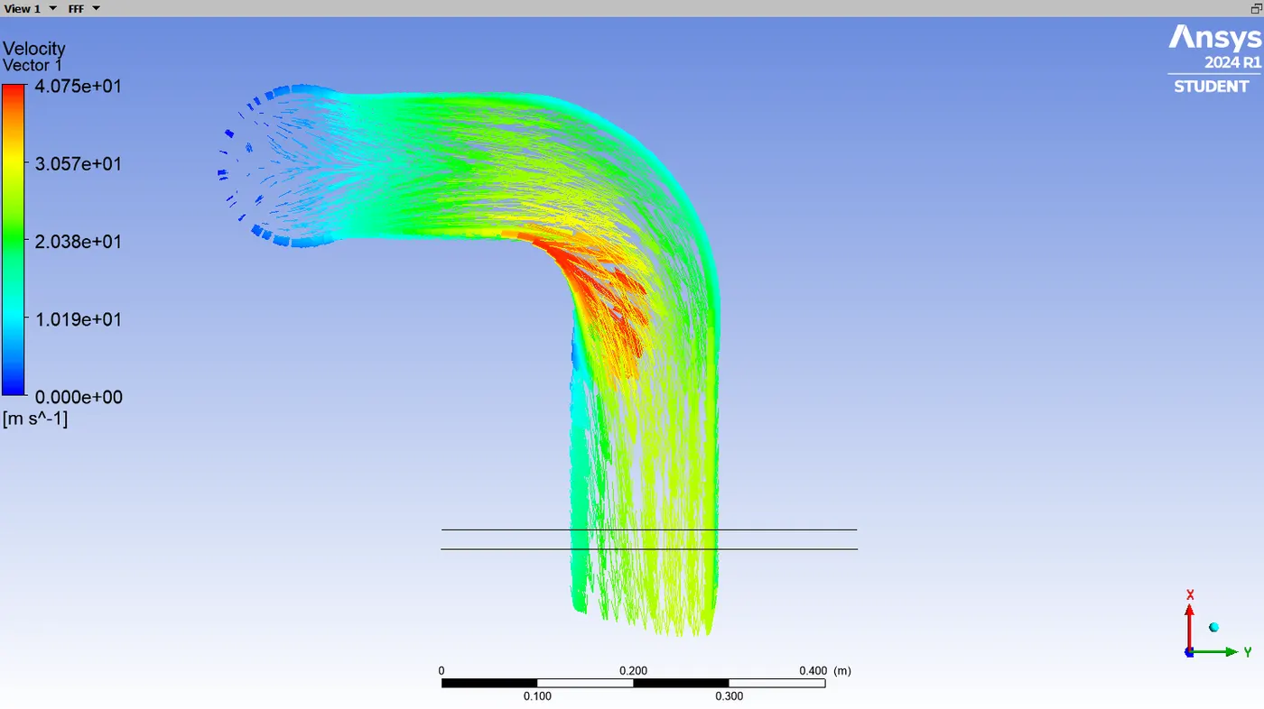
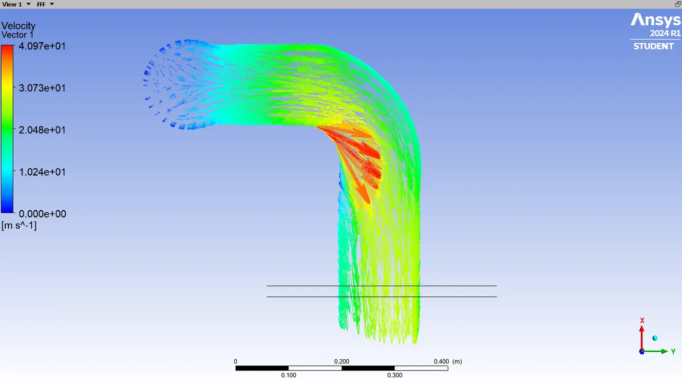
• you can see the fluid flow direction and temperature of the fluid through the velocity vertex in plane 1.

    

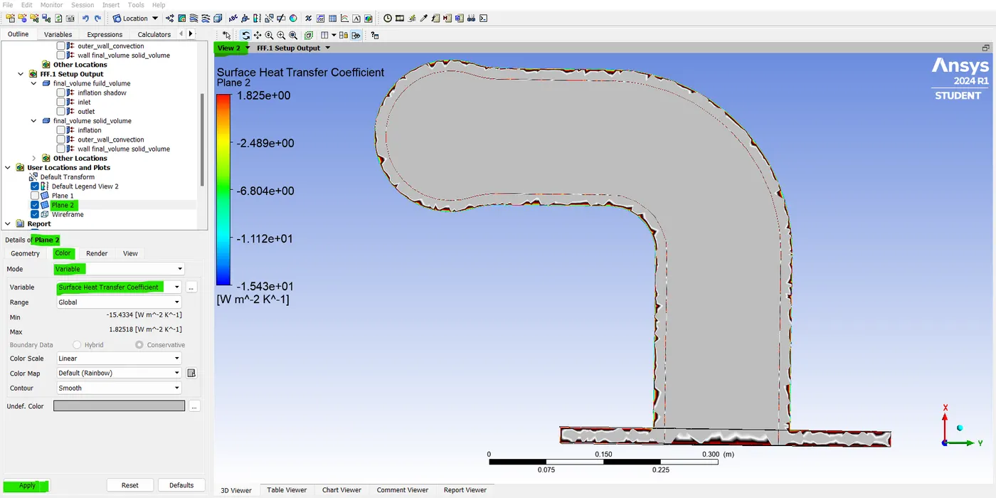
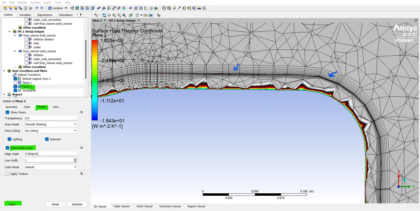
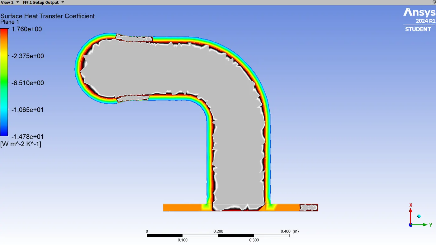
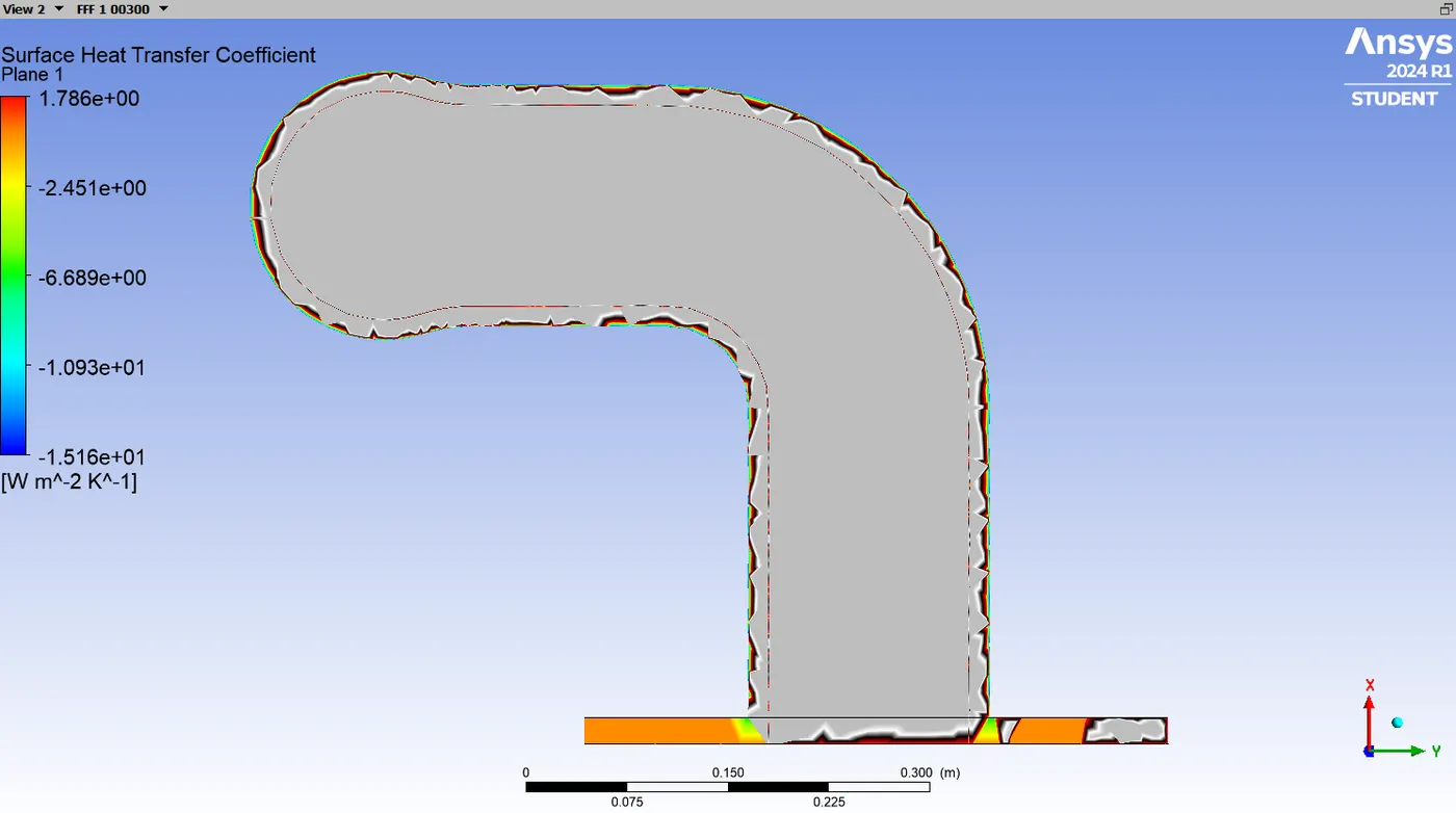
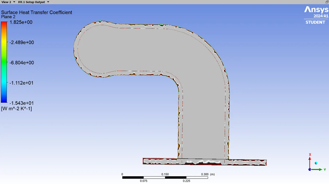
• Now you can see the surface heat transfer coefficient is a quantity that is always available only in the first cell that is attached to the wall. so, that is why we added the inflation layer. so, here we are getting this very smooth-looking plot that shows the high value of the heat transfer coefficient at this location. which means the majority of the mesh is within the inflation layer. so, the surface heat transfer coefficient is highest in this particular location.  

     

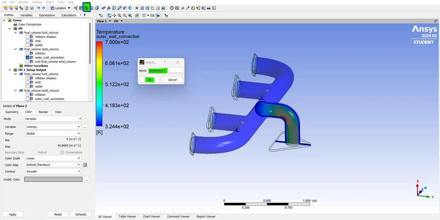
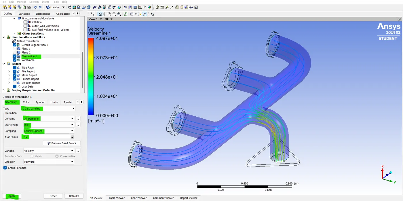
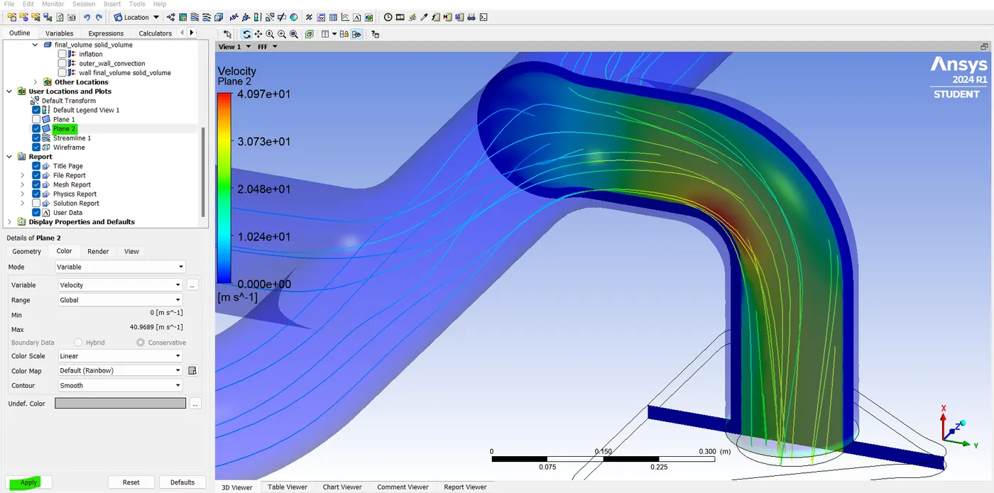
• now we are going to add the strime lines so, select the timeline. and then I'm going to start the streamlines from our inlets they are going to be having about 25 streamlines and they are going to be about 25 streamlines and they are going to be colored by a velocity. so, let's click "ok".
• so, let's see the velocity is really low in this section (inlet). and the velocity is very high in this section (outlet). why because of mass conservation. so, here you have a particular mass flow rate. right now, all of these diameter are very similar. it means the velocity on all these four faces is pretty much the same. and area time velocity is the flow rate the volumetric flow rate and there is a four inlets and then there this only one outlet all that air needs to flow out which means the velocity there is going to be very high.
• now remember it is a steady state simulation which means the air that comes through the outlet is always going to have a higher velocity. now because of this higher velocity, what going to happen is we will have a higher Reynolds number there which means we should have a higher heat transfer coefficient. which means there is going to be more heat transfer. from the fluid to the solid. and that's why the solid temperature in that location is higher.

Result:

Plots:-

Case-1

Default mesh size:- 225 mm.

Baseline mesh size:- 50 mm.

No.of.inflation layer:- 0.

Residual plot:

 

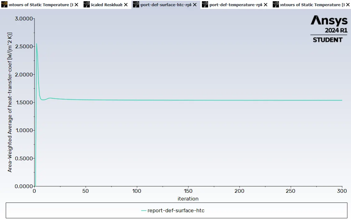
Heat transfer coefficient plot:

 

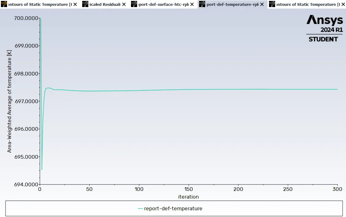
Temperature at external pipe wall plot:

 

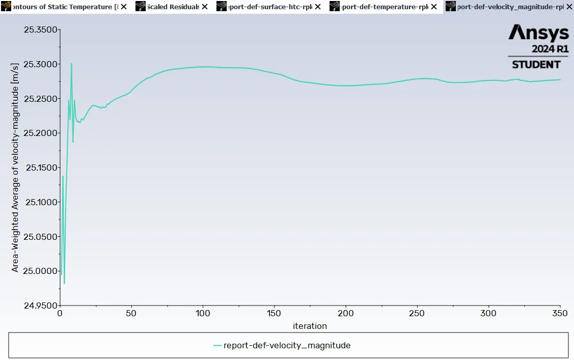
Velocity magnitude:

view-1:

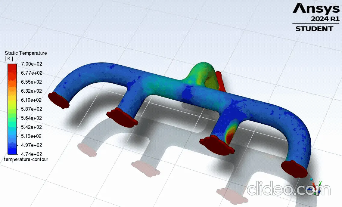
Temperature contour plot:

view-1:

 

pressure contour plot:

view-1:

 

velocity contour:

view-1:

 

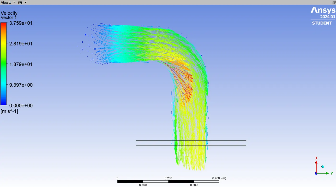
velocity vector:

view-1:

 

HTC Plot:

view-1:

 

Case-2 

Default mesh size:- 200 mm.   

Baseline mesh size:- 30 mm.

No.of.inflation layer:- 12.

Residual plot:

 

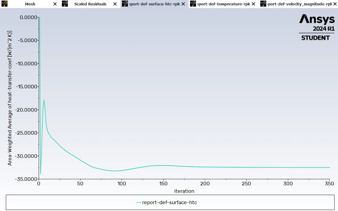
Heat transfer coefficient plot:

 

Temperature at external pipe wall plot:

 

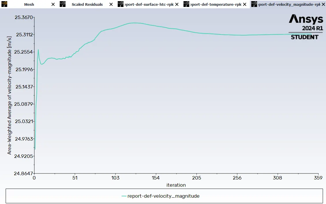
Velocity magnitude:-

Temperature contour plot:

view-1:

 

pressure contour plot:

view-1:

 

velocity contour:

view-1:

 

velocity vector:

view-1:

 

HTC Plot:

view-1:

 

Case-3

Default mesh size:- 100 mm.

Baseline mesh size:- 12 mm.

No.of.inflation layer:- 7.

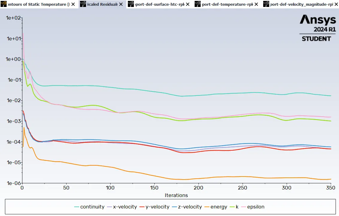
Residual plot:

 

Heat transfer coefficient plot:

 

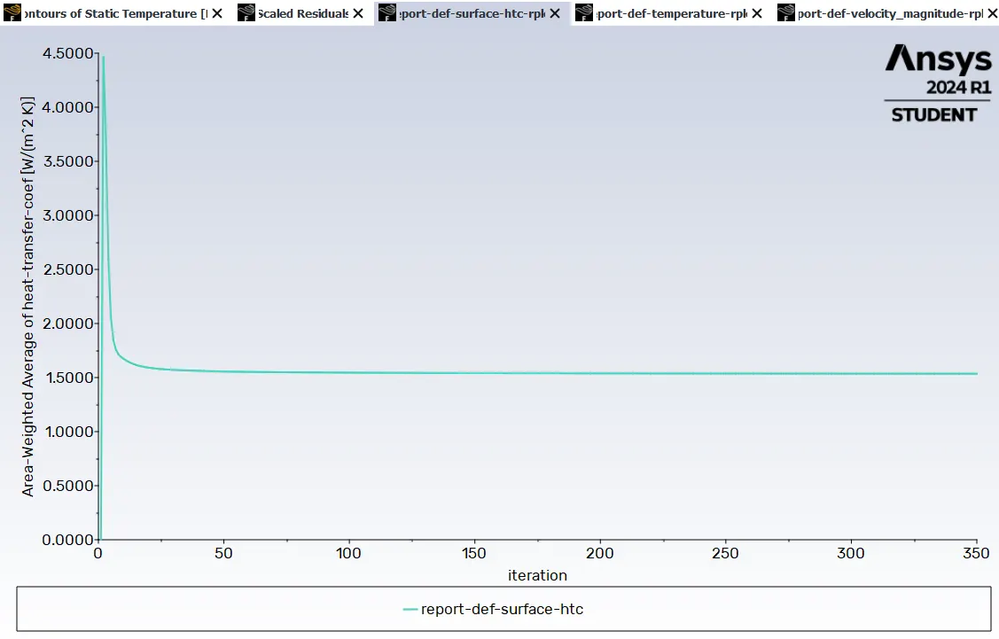
Temperature at external pipe wall plot:

 

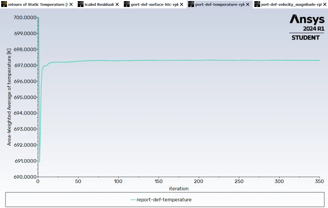
Velocity Magnitude:

view-1:

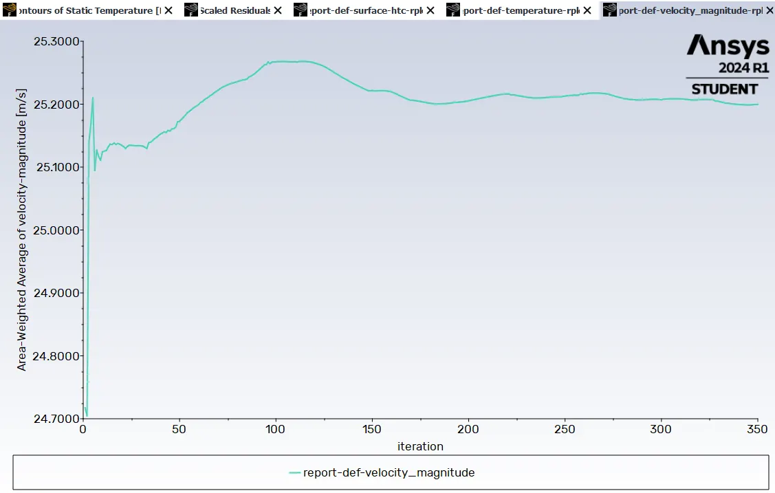
Temperature contour plot:

view-1: 

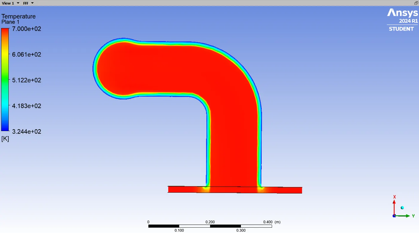
pressure contour plot:

view-1:

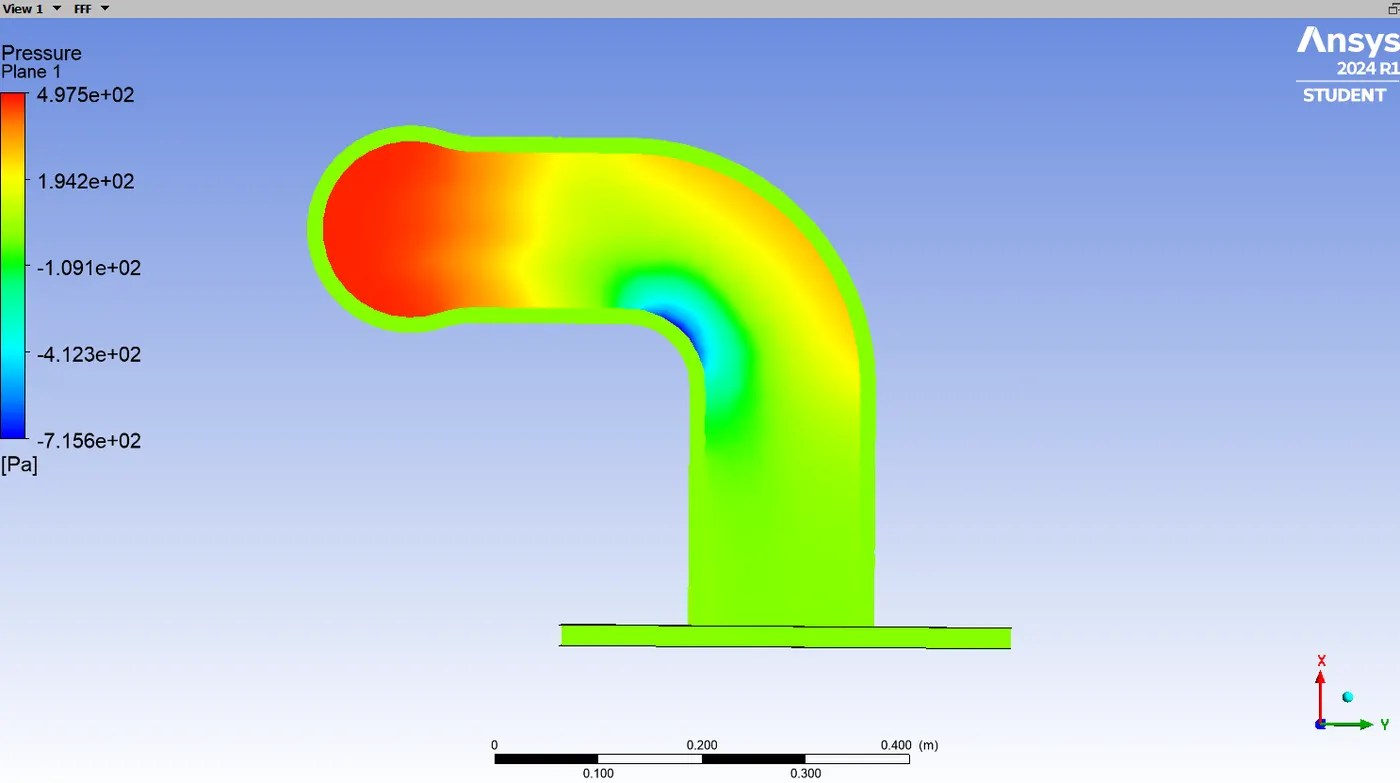
velocity contour:

view-1:

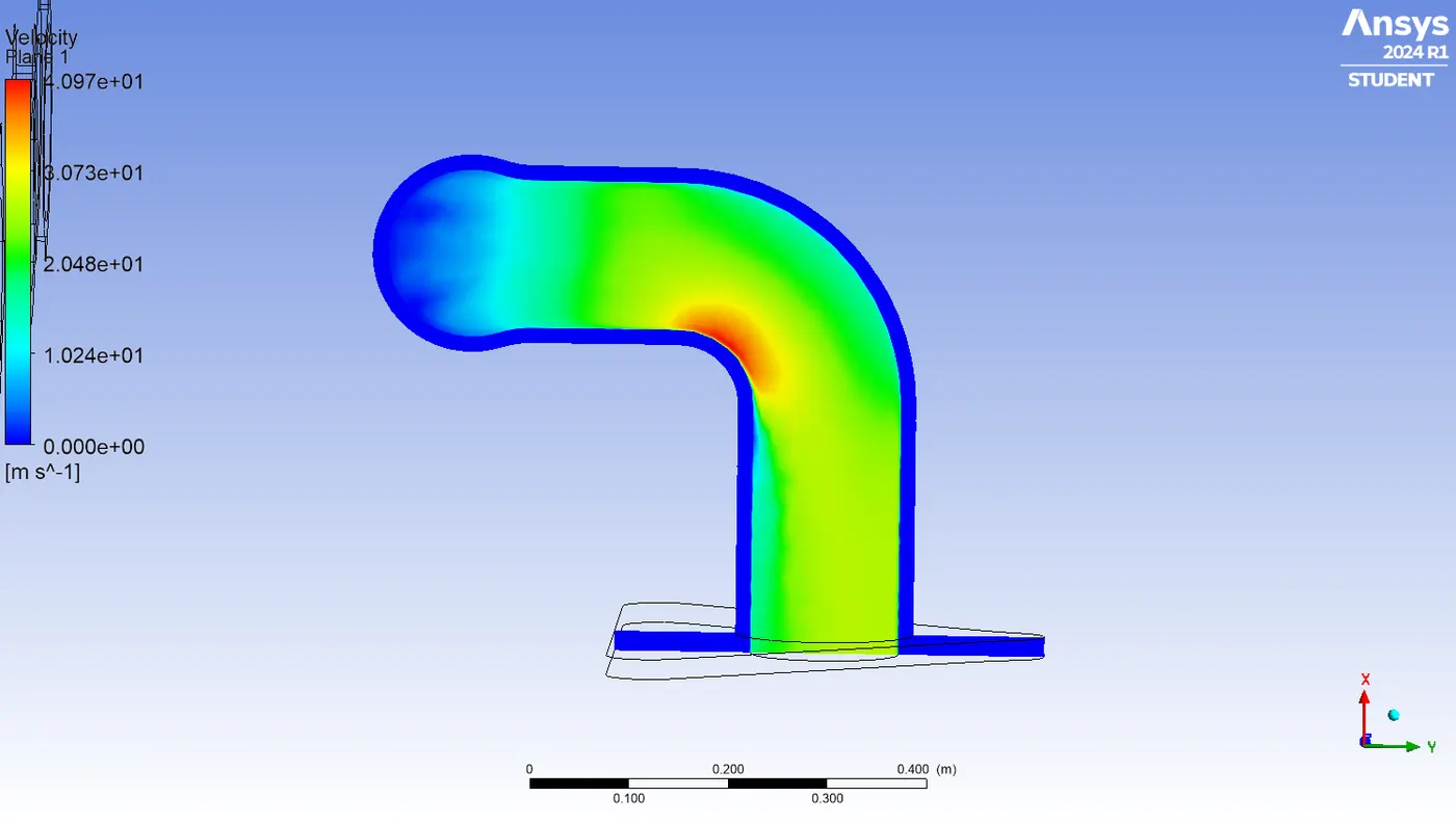
velocity vector:

view-1:

 

HTC Plot:

view-1:

Baseline mesh Animation:

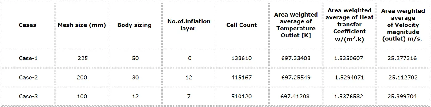
Grid Independence test:  

 

How would you verify if the HTC prediction from the simulation is right? On what factor does the accuracy of the prediction depend? 

1. so to verify whether the HTC Predictions are right or not we can perform several cases with different sizes and different boundary conditions if the solution is converged at the same point and also refering studies related to the analysis and then we can predict whether the simulation values are right. so this is one of the ways to predict the values.
2. Another way is we need to run an experiment and then we can verify the numerical result with experiment results. so, running the experiment is a time-consuming process and also expensive. so that we have an analytic equation which is in algebraic form. and we can verify the numerical result with analytical results. The sample calculation for case-2 analytic results is attached at the top of this report similarly, we need to follow for case 1 and case 3.

Conclusion:

• There are notable changes in the three cases, so the mesh is more refined from cases 1 to 3 to check the grid dependence. So, the refined mesh generates a smooth contour plot near the wall due to the presence of a lower Y+ value.
• At the tube bend region, the fluid flow parameters are better solved for the refined mesh. Hence the smoother mesh provides accurate results, in all 3 cases we conclude that case 3 is more refined at a lower element size.
• The velocity magnitude increases with no.of.elements so we can take the 25.399704 m/s as the final velocity magnitude.   
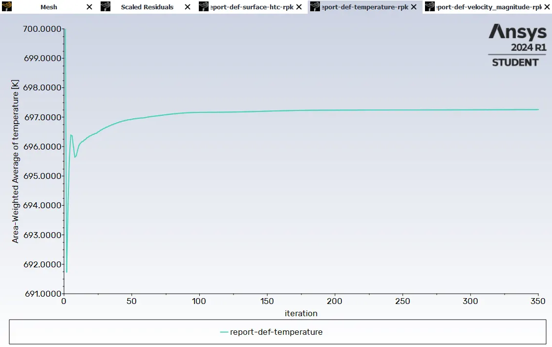
• The temperature also increases at the outlet when the no.of.element is increasing. The HTC plot has also increased slightly. the change is also negligible.
• The Appropriate mathematical model that is turbulence model should be used to capture the flow parameters correctly that is for no-slip conditions we used the k-epsilon model.