Week 4 - CHT Analysis on Exhaust port

Aim:- To study the Conjugate Heat Transfer Analysis of Exhaust Port using ANSYS Fluent.

Objective:-

• Simulation of Conjugate Heat Transfer on exhaust manifold.
• Calculation of wall heat transfer on internal solid surface.
• Maintaining appropraite y+ value for the turbulence model.

Conjugate Heat Transfer (CHT) refers to the simultaneous analysis of heat transfer in both solid structures and adjacent fluids. It is a computational technique used in engineering simulations to model and understand the thermal interactions between different domains, such as solid materials and surrounding fluids, within a single simulation framework.

In many practical engineering applications, heat transfer occurs across boundaries between solids and fluids. For example, electronic components dissipate heat into the surrounding air, combustion chambers transfer heat to the walls, or coolant flows through channels in contact with solid structures. Conjugate Heat Transfer analysis accounts for these coupled heat transfer phenomena, providing a more realistic representation of thermal behavior in complex systems. This approach is employed when there is a need to understand the thermal interaction between different domains, such as solids and fluids, within a single simulation framework.

The key components of Conjugate Heat Transfer analysis include:

1. Solid Domain:- This represents the solid structures or components involved in the analysis, such as walls, heat sinks, or any other solid material where heat is generated or transferred.

2. Fluid Domain:- This represents the fluid or gases surrounding the solid structures, where heat transfer occurs through convection. The fluid can be in motion, and its temperature distribution is influenced by heat exchange with the solids.

3. Interface or Boundary:- The interface between the solid and fluid domains is where the heat transfer occurs. It considers the thermal interaction between the two domains, taking into account conduction through solids and convection between solids and fluids.

Conjugate Heat Transfer simulations involve solving coupled equations for heat conduction in solids and heat convection in fluids simultaneously. This integrated approach allows engineers to study the temperature distribution and heat transfer characteristics across the entire system.

Applications of Conjugate Heat Transfer analysis are diverse and include fields such as electronics cooling, automotive engineering, aerospace, energy systems, and more. By providing a comprehensive understanding of thermal behavior in complex systems, CHT simulations aid in optimizing designs for improved performance and reliability.

The primary reasons for conducting Conjugate Heat Transfer analysis include:-

1. Coupled Heat Transfer Phenomena:- CHT is crucial when dealing with systems where heat transfer occurs across multiple materials or phases, such as the heat exchange between a solid component and a surrounding fluid.

2. Realistic Simulation:- In many engineering applications, particularly those involving complex thermal systems like electronics cooling, combustion chambers, or heat exchangers, it is essential to account for the interaction between solid structures and surrounding fluids for a more accurate and realistic simulation.

3. Temperature Distribution Prediction:- CHT enables engineers to predict the temperature distribution within both solid and fluid domains, allowing for a more comprehensive understanding of the thermal behavior of the entire system.

4. Performance Optimization:- By simulating the conjugate heat transfer, engineers can optimize the design of components to enhance thermal performance, ensuring that temperature constraints and thermal management requirements are met.

5. Multidisciplinary Analysis:- Conjugate Heat Transfer analysis is often integrated into multidisciplinary simulations where thermal considerations are critical, such as in the aerospace, automotive, electronics, and energy industries.

CHT simulations can be applied in various fields, including:-

• Electronics Cooling:- Studying the heat dissipation in electronic components like integrated circuits and heat sinks.
• Automotive Engineering:- Analyzing the thermal behavior of engine components, exhaust systems, and cooling mechanisms.
• Aerospace:- Investigating heat transfer in components like turbine blades, spacecraft re-entry, or thermal protection systems.
• Renewable Energy:- Understanding heat transfer in solar collectors, geothermal systems, or wind turbine components.
• Biomedical Engineering:- Analyzing the thermal behavior of medical devices or the interaction of tissues with external heat sources.

Conjugate Heat Transfer analysis provides valuable insights into the thermal performance of systems and aids in the design and optimization of engineering applications where heat transfer is a critical factor.

Geometry:-

Importing the downloaded geomerty in the spaceclaim and extracting the fluid volume, where the fluid will interact with the exhaust port.

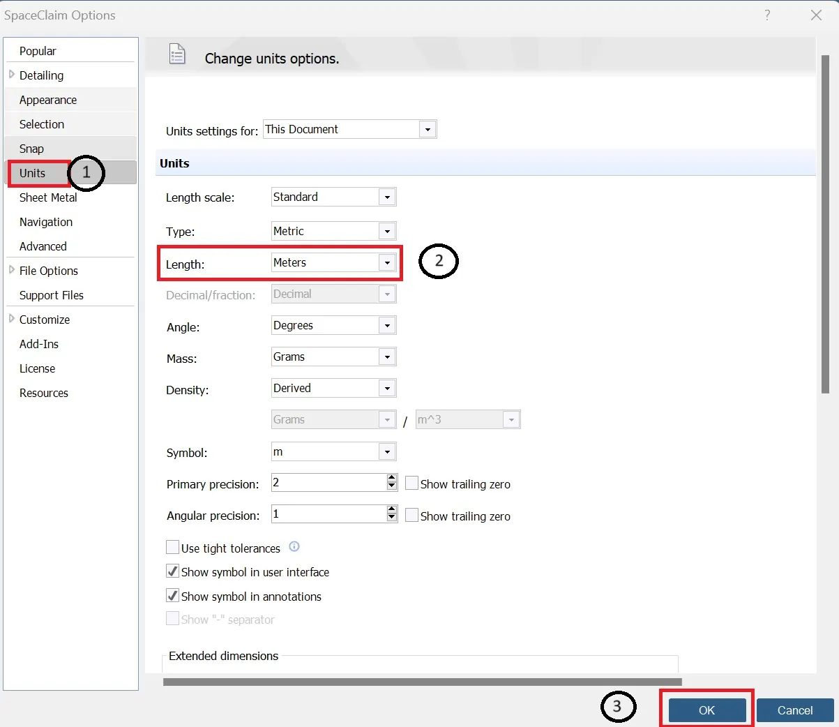
1. Changing the units in File-> Units -> Length -> Meters -> OK.

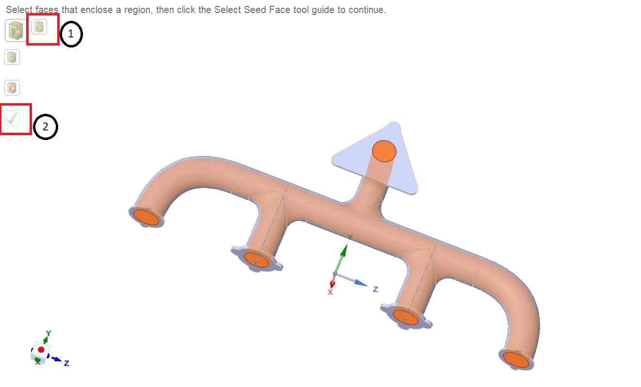
2. Go to Prepare -> Volume extract -> Select edge and select the edges at inlet and outlet and complete to get

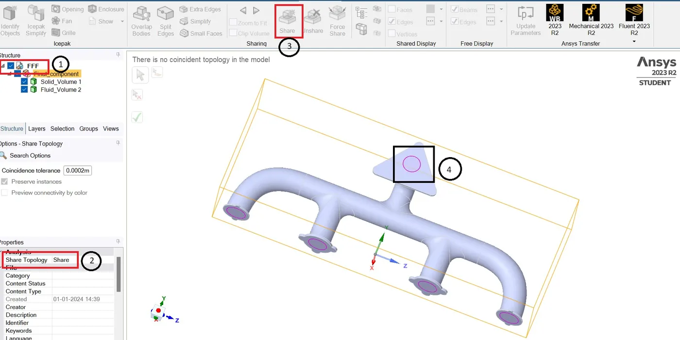
Go to the FFF -> share topology -> share -> Workbench -> Share and then we get this purple circles at inlet and outlet.

Mesh:-

Named selection

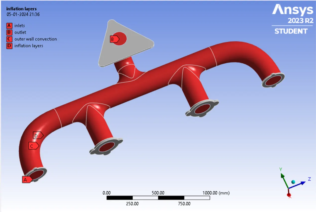
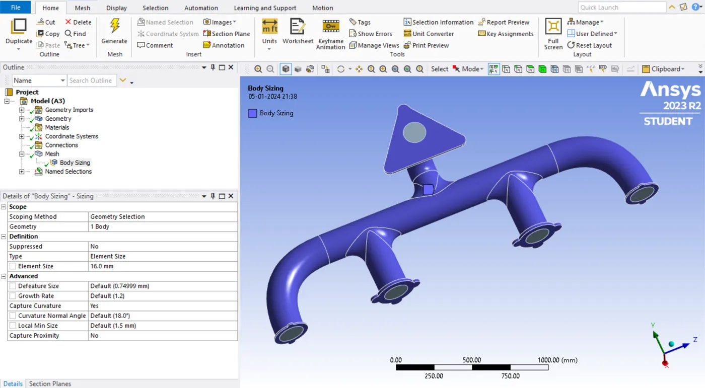
Right click on Mesh -> Insert -> Sizing and select the body selection tool and select the whole body and insert element size as 16 mm and capture curvature as yes

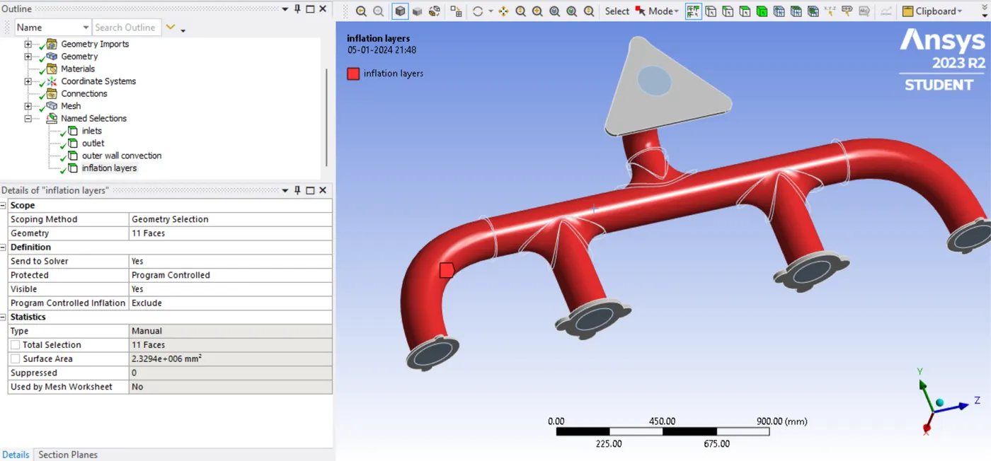
We hide the outer solid volume and name the inner fluid volume as Inflation layers

Mesh:-

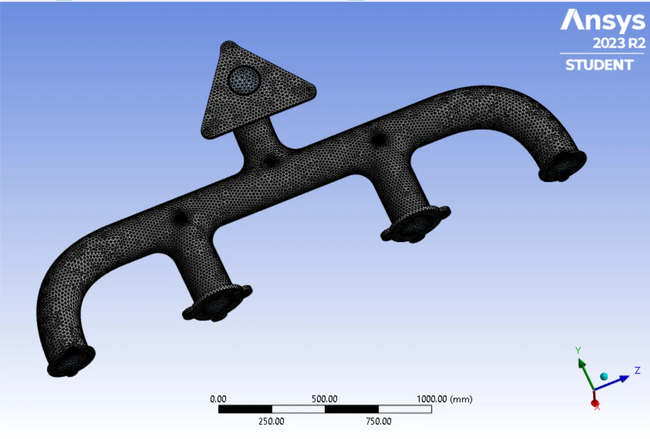
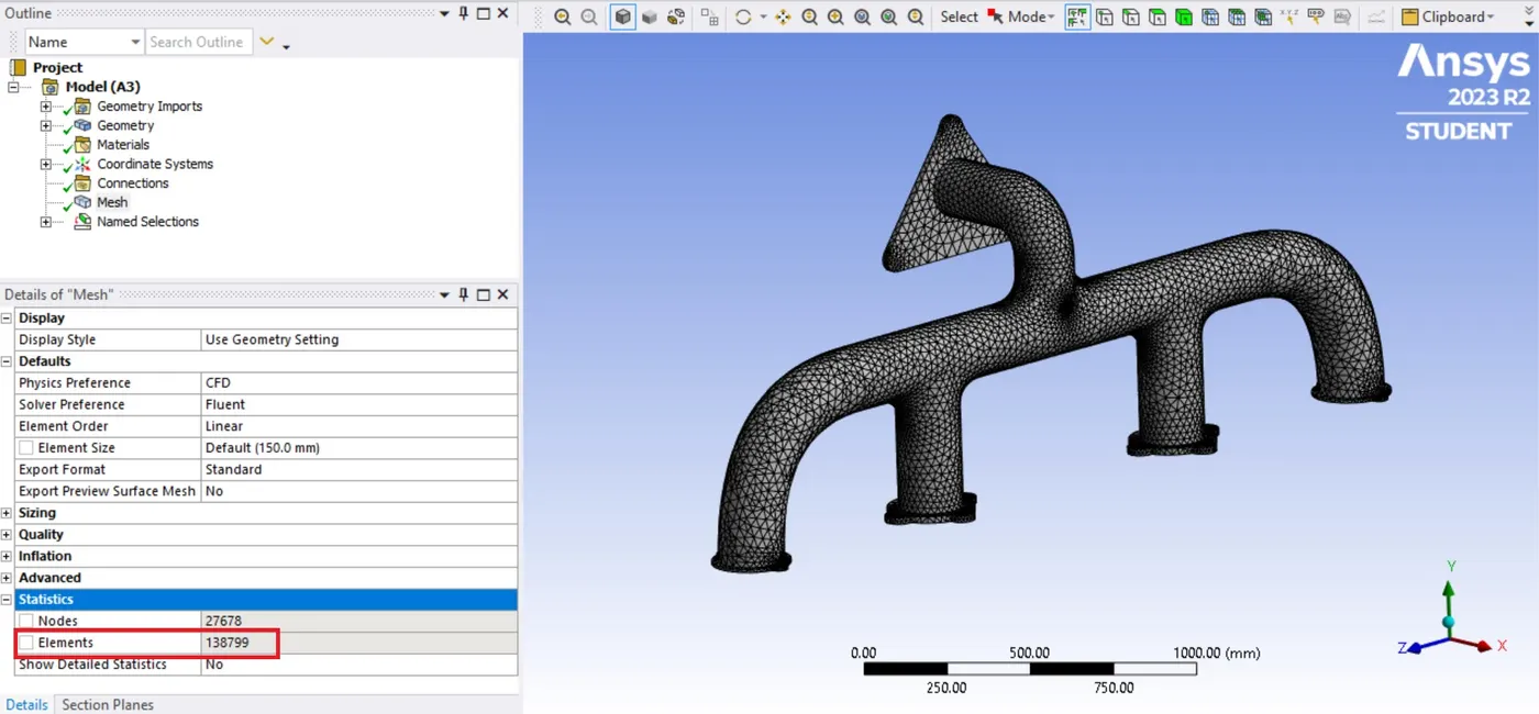
Om generating the mesh, we get mesh with cell count as 138799

Solver:-

Here, we will be using the Double Percision in Solver options 4 Solver Processes and we start,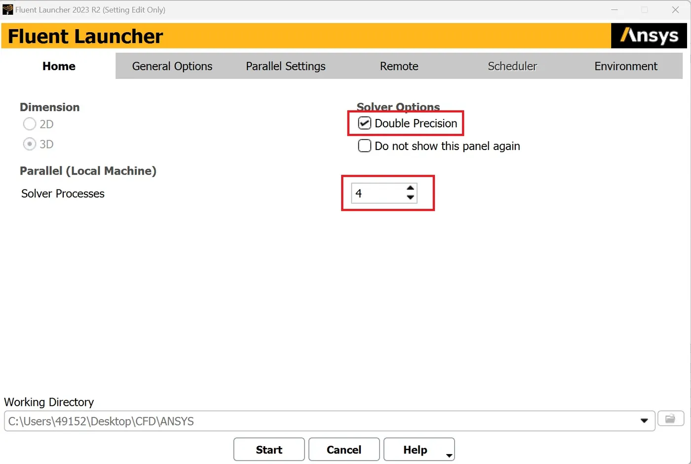

Refined mesh with inflation layer

We add inflation layer by going into Inflation -> All faces in chosen Named selection (in Use Automatic inflation) -> inflation layer (in Named selection) -> Total thickness (in inflation Option) -> 5 (in number of layers)

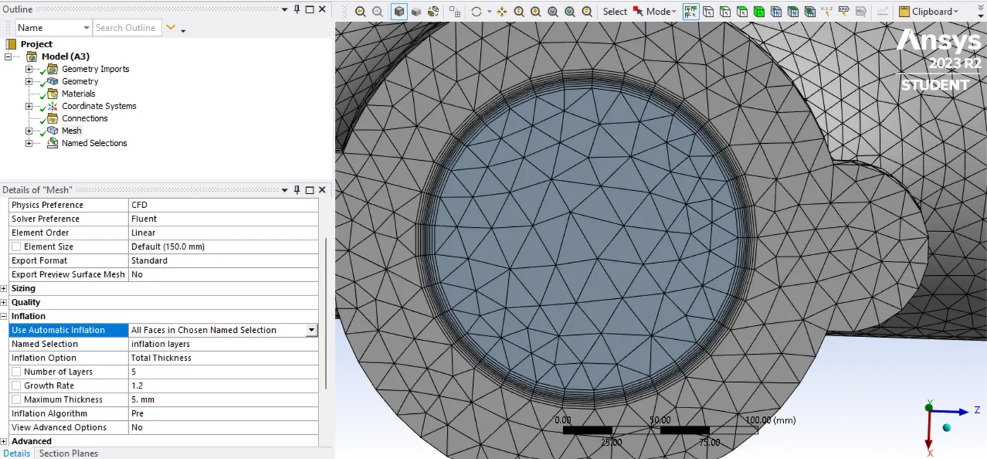
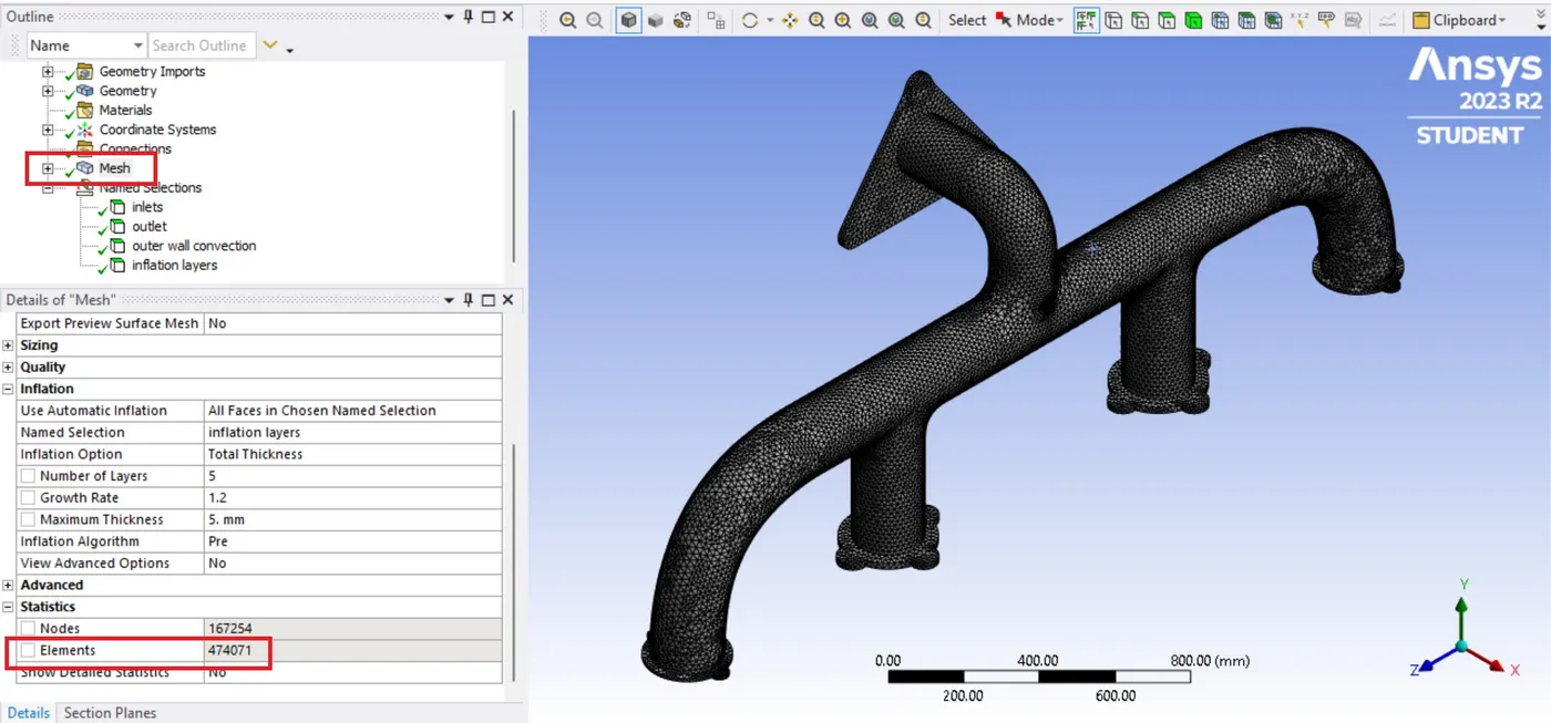
On generating the mesh, we get mesh as following with the element size of 474071

Solver:-

Here, we will be using the Double Percision in Solver options 4 Solver Processes and we start,

Solver:-

• Solver -> Pressure based solver
• Solver state -> Steady state
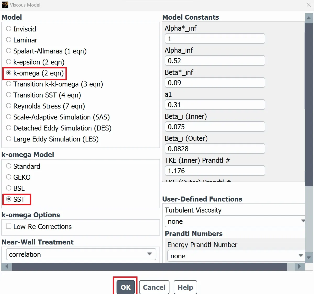
• Turbulence Model -> K-Omega, SST

Boundary Conditions:-

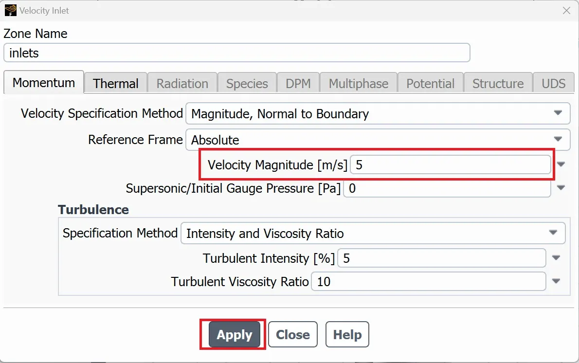
• Inlet velocity -> 5m/sec
• Heat Transfer Coefficient -> 20 W/m^2 K
• Pressure outlet -> 0 Pascals

Go into the Physics -> Models -> click on Energy -> viscous -> K-Omega -> SST -> OK

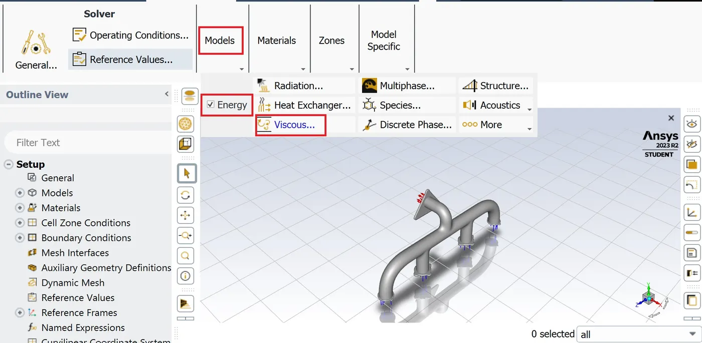
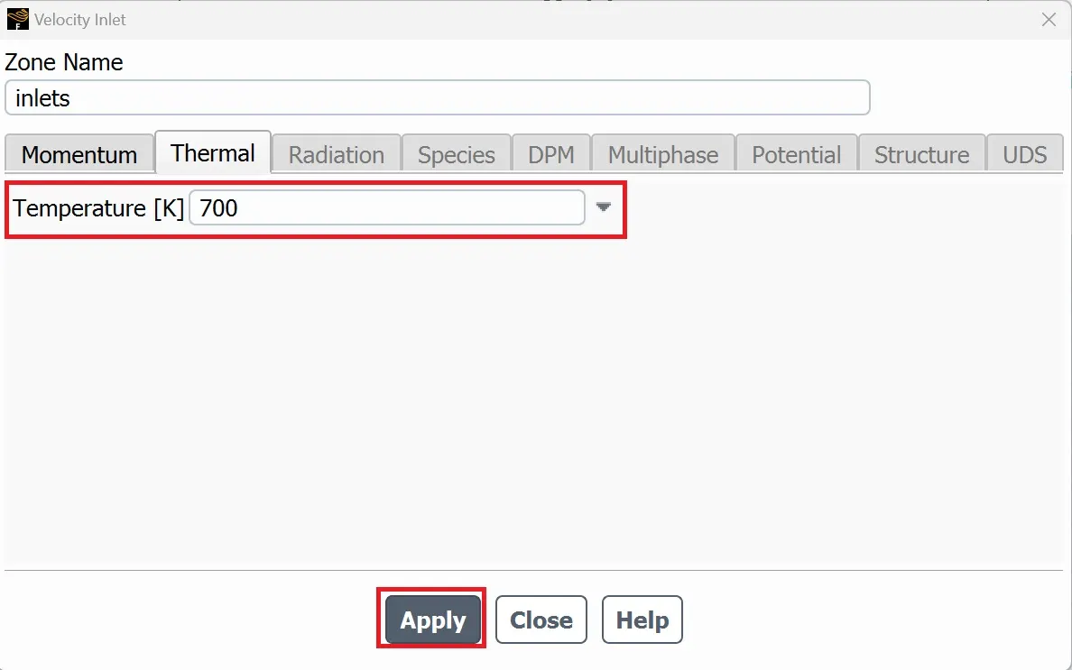
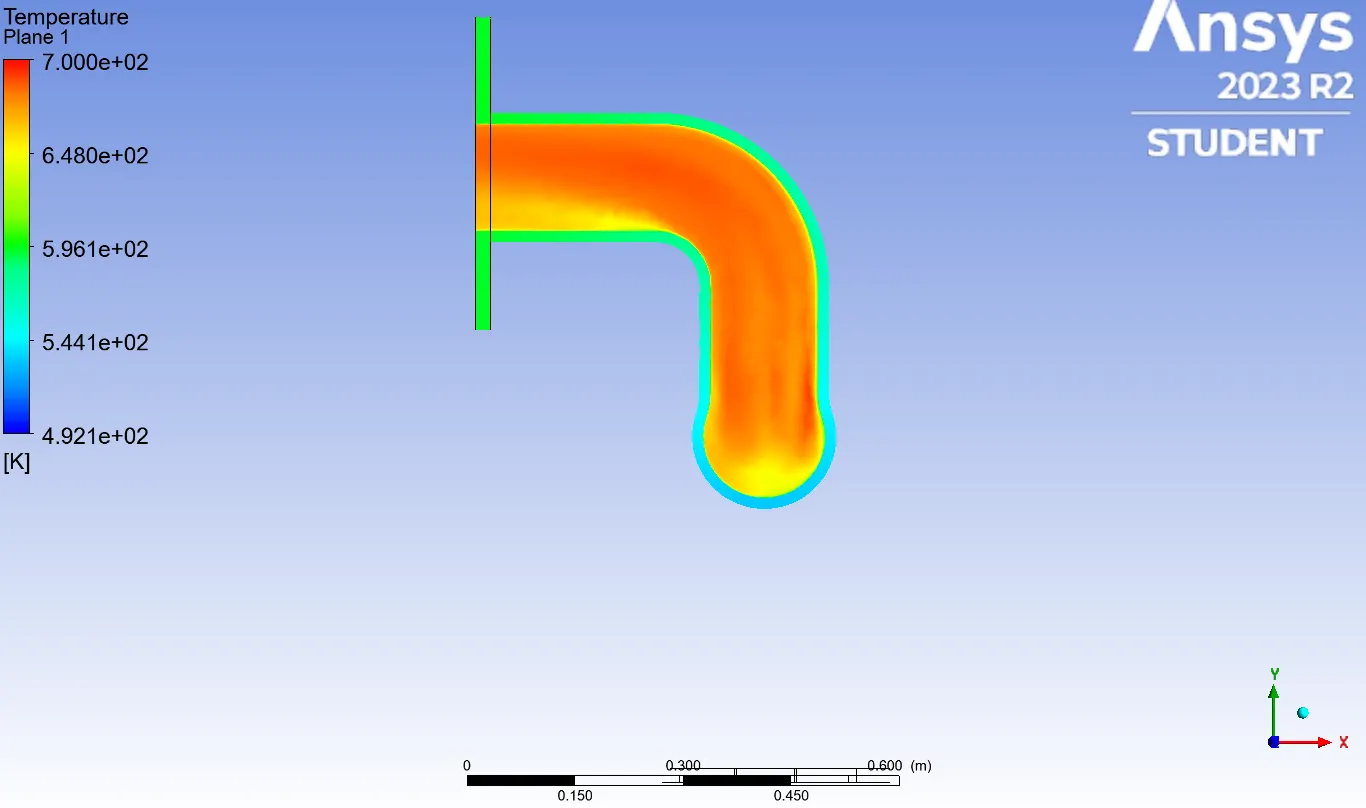
Go into Zones -> Boundary -> inlet -> edit -> inlet velocity as 5 m/sec -> Temperature -> 700K

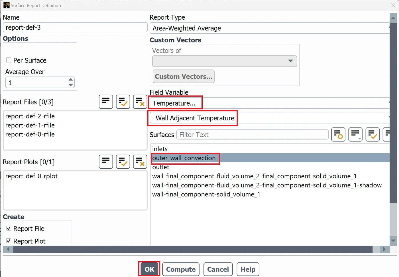
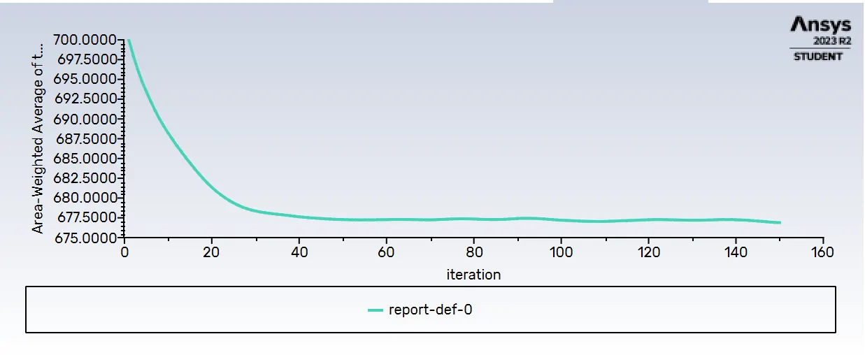
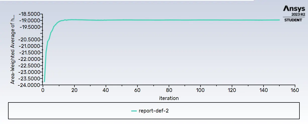
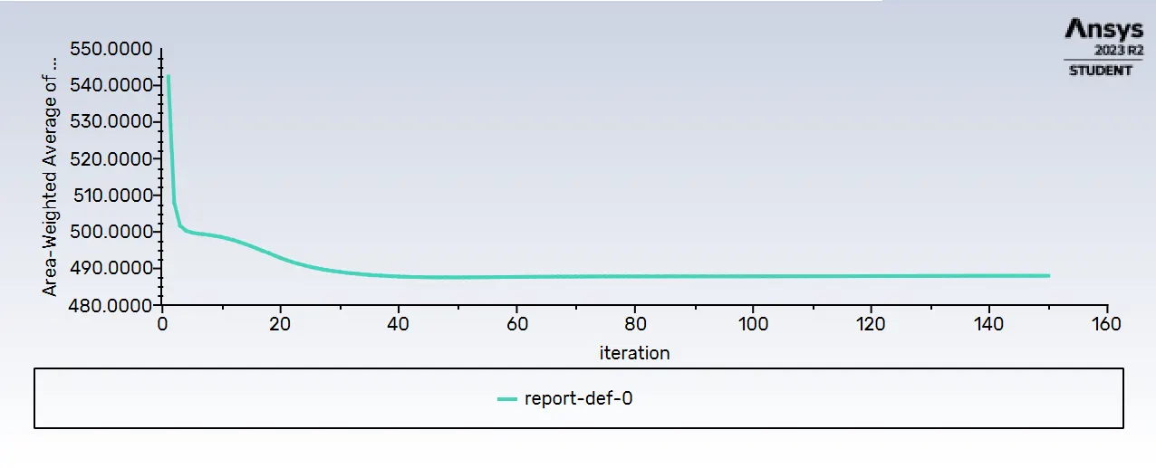
For the report, we go into solution -> definations -> New -> Surface report -> Area Weighted Average

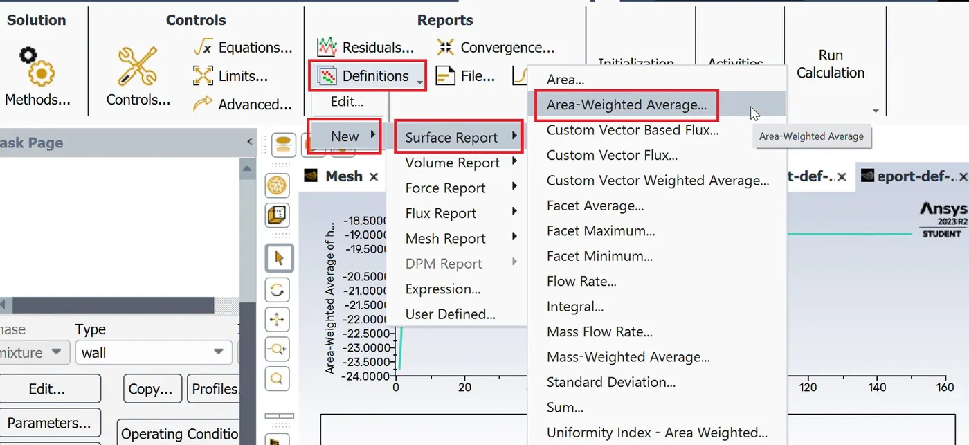
In Surface Report Defination -> change Field Variable to Temperature -> Wall Adjacent Temperature -> Outer_Wall_Convection

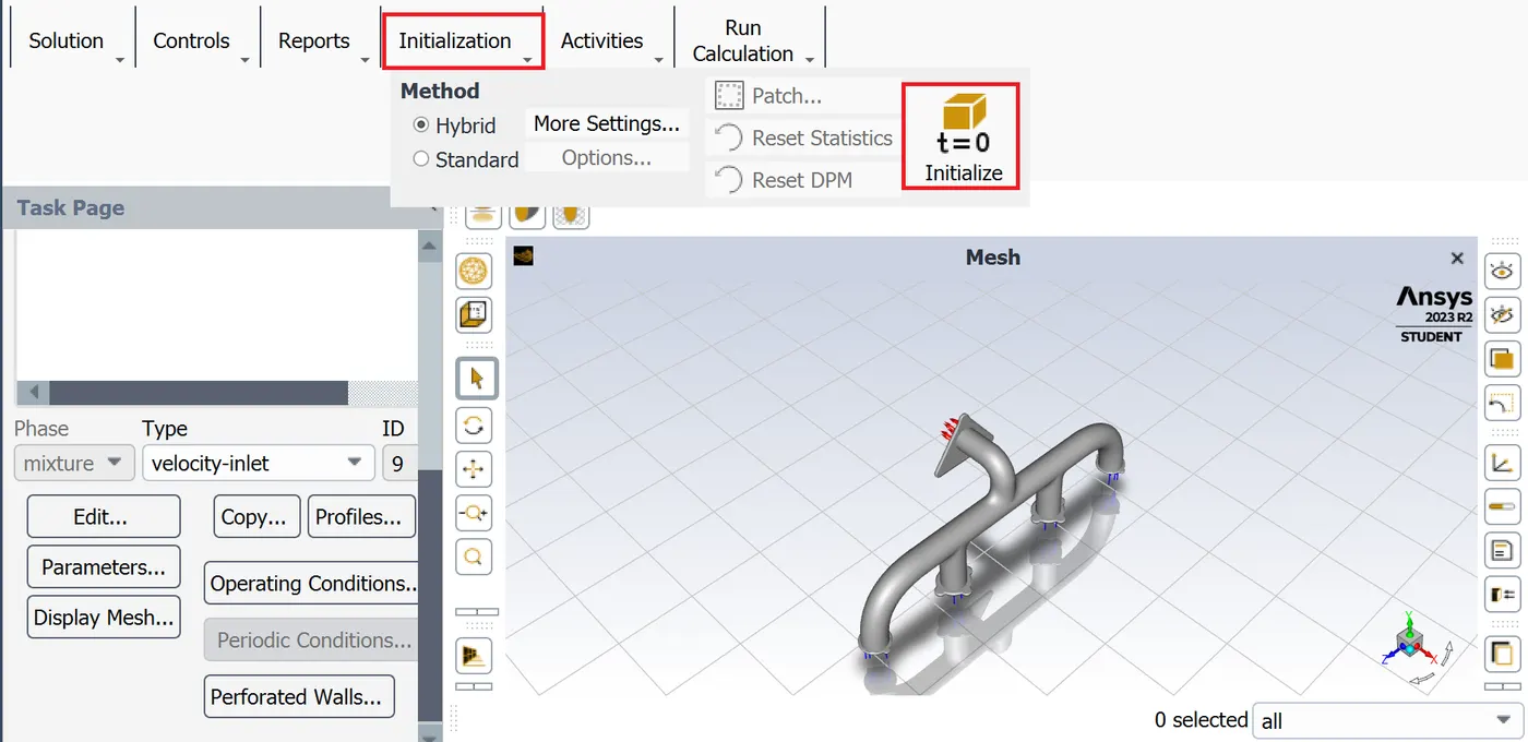
Go into Solution -> Initialization -> Initialize

Result:-

Results with Infation layers

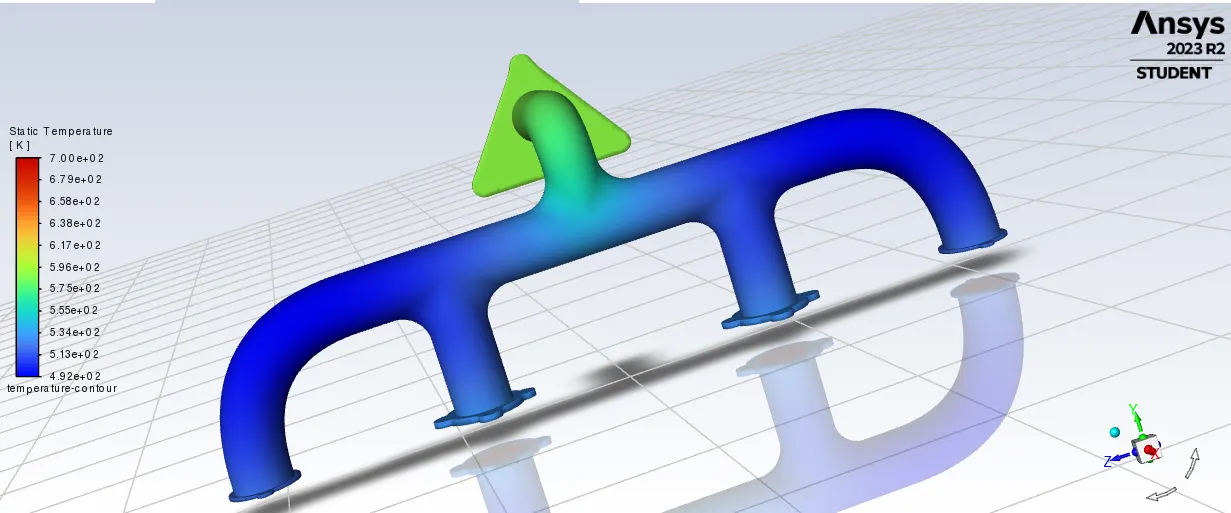
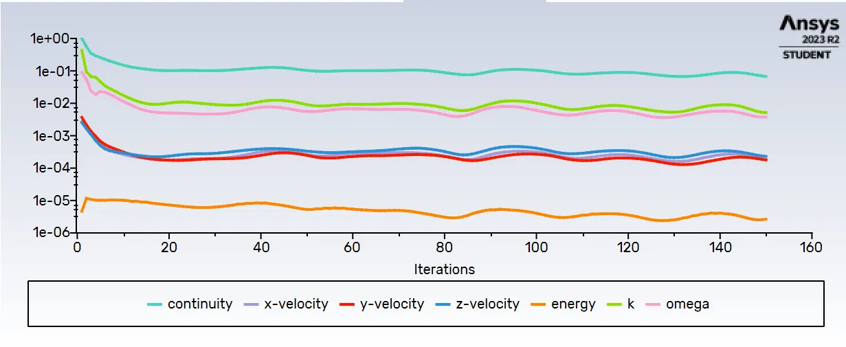
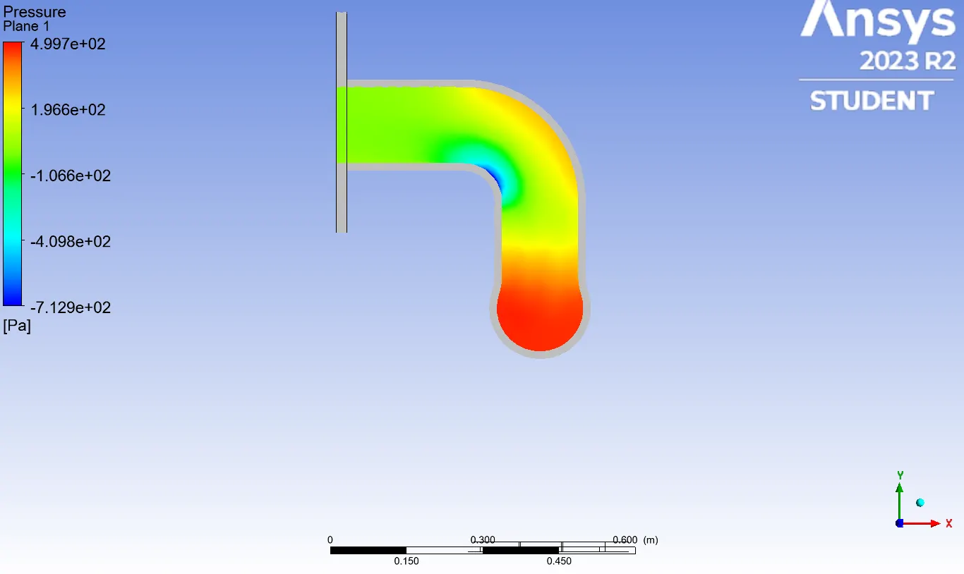
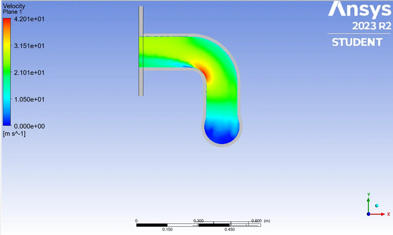
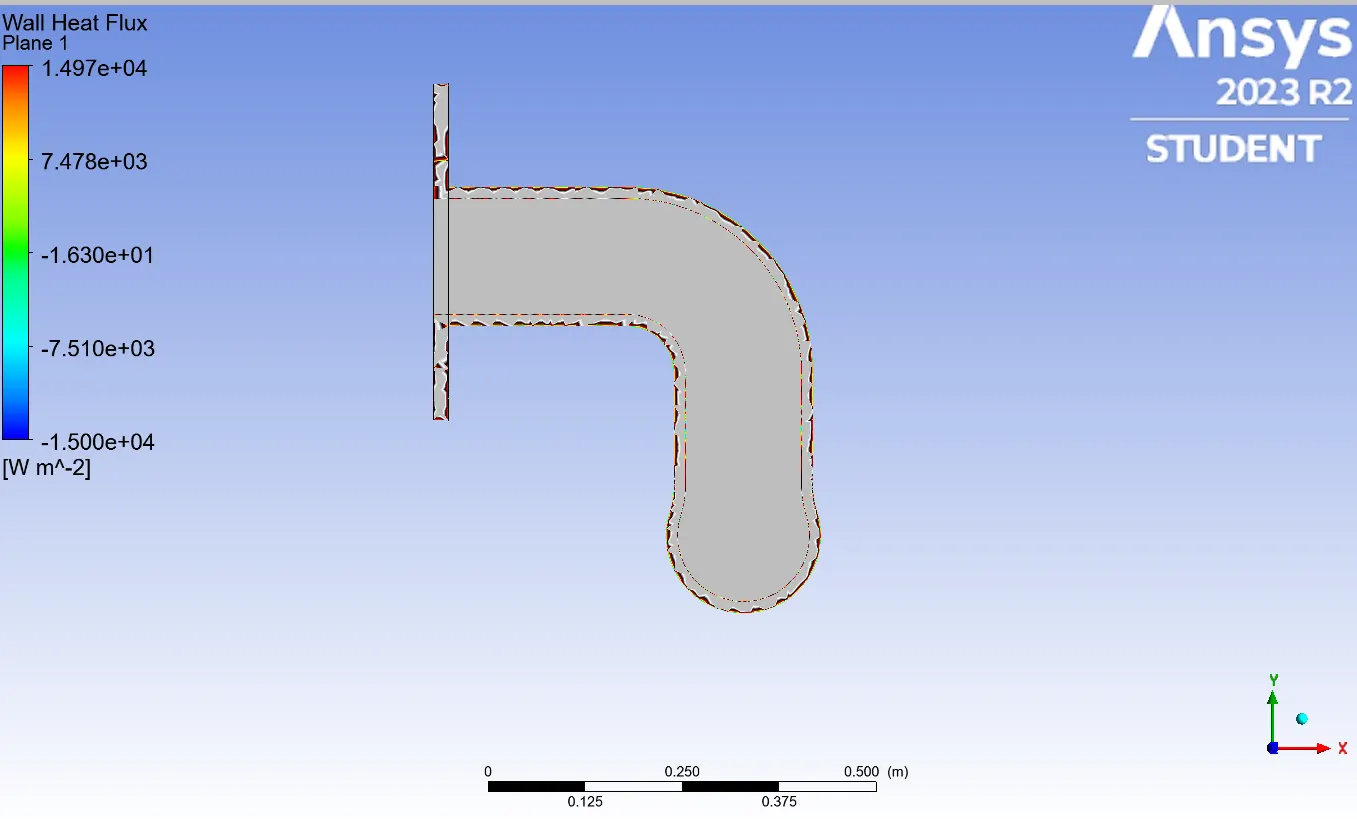
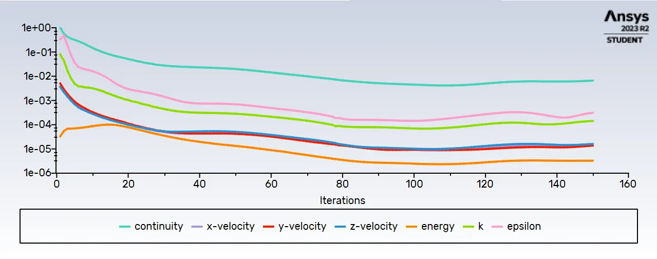
Then we run it for 150 Iterations and we get the following results,

Residual plot:-

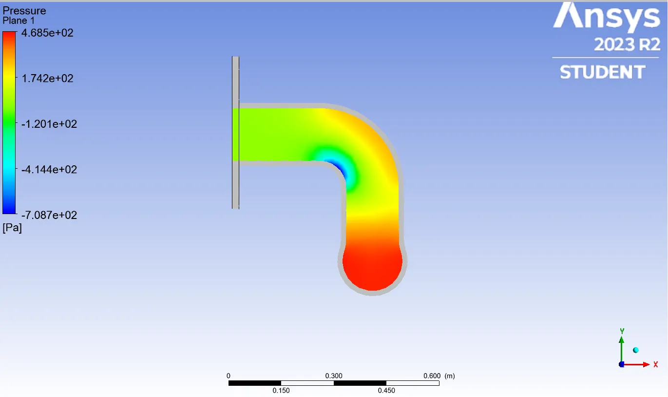
Pressure Contour:-

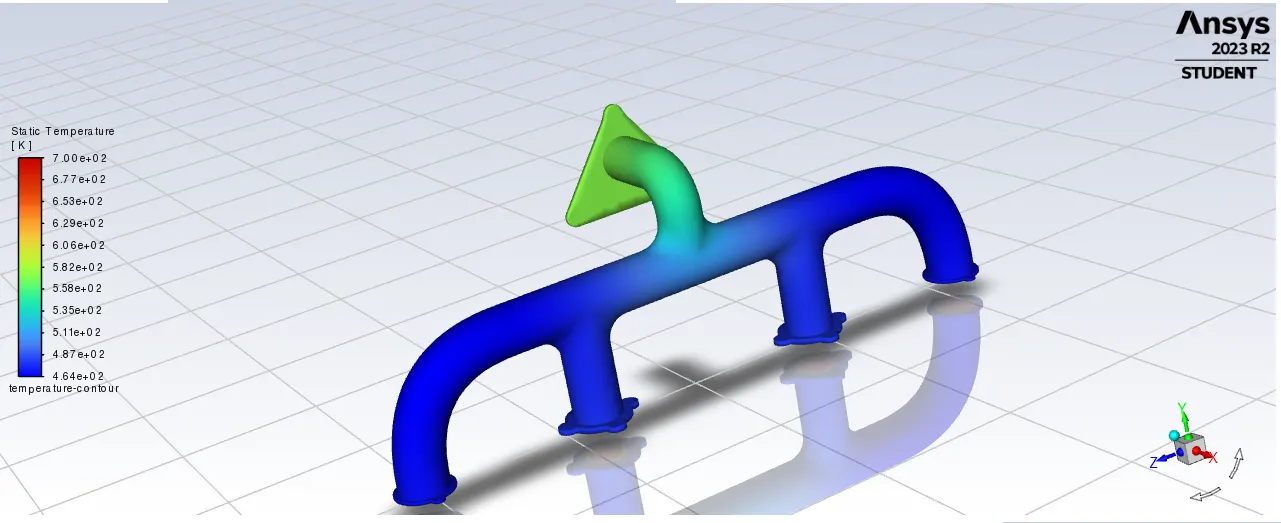
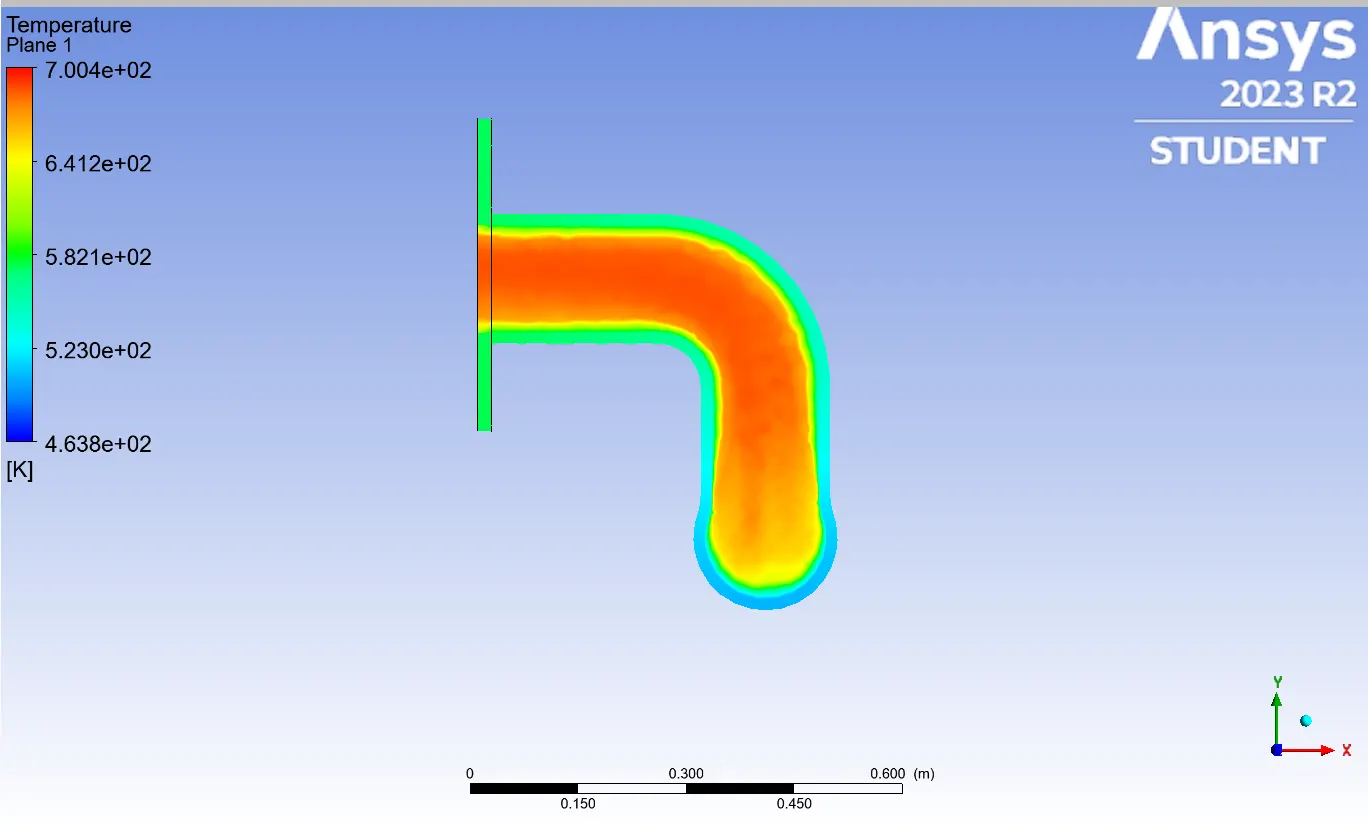
Temperature Contour:-

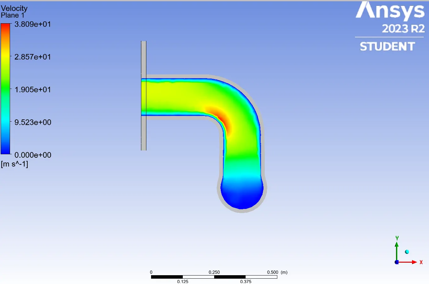
Velocity Contour:-

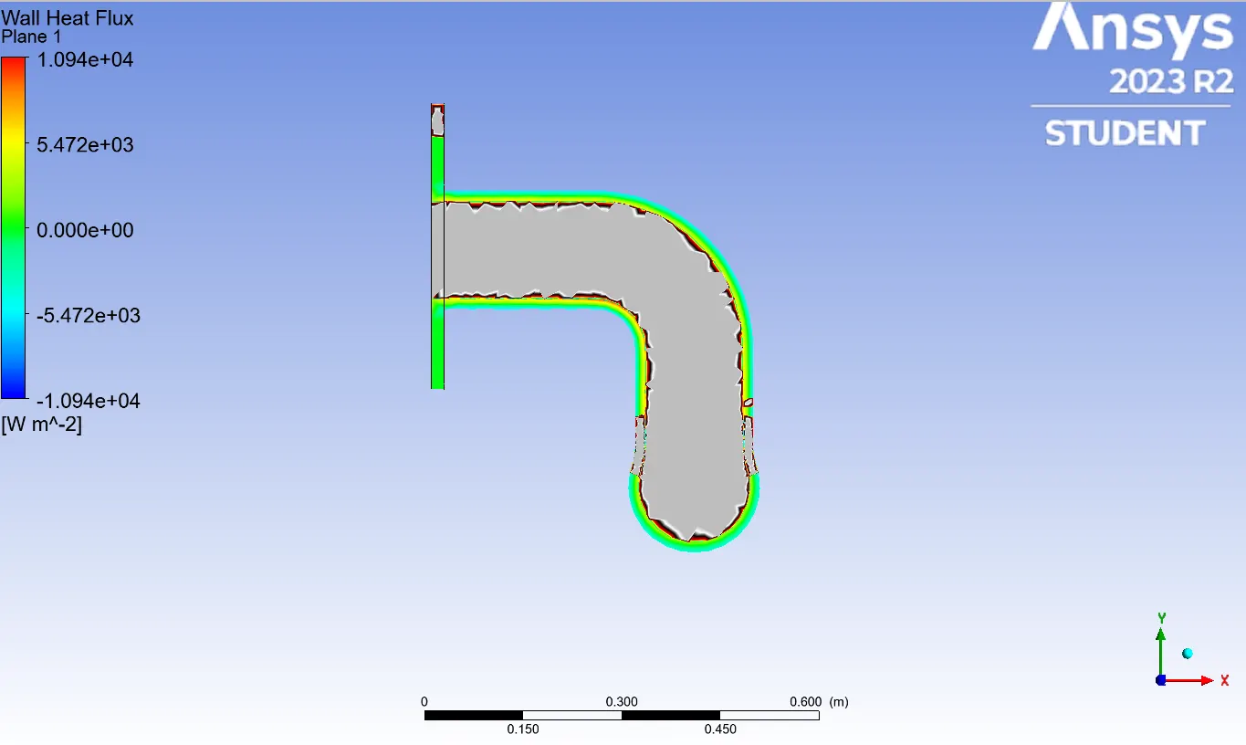
Wall Heat Flux Contour:-

Results:-

Without inflation layers

Residual plot:-

Pressure Contour:-

Temperature Contour:-

Velcoity Contour:-

Wall Heat Flux Contour:-

Nusselt number is given by:-

The Nusselt number (Nu) is a dimensionless number used in fluid mechanics and heat transfer to quantify the convective heat transfer between a fluid and a solid surface. It represents the ratio of convective to conductive heat transfer across the fluid-solid interface. The Nusselt number is named after the German engineer Wilhelm Nusselt, who made significant contributions to the study of heat transfer.

The Nusselt number is defined differently for different modes of heat transfer, such as natural convection, forced convection, and condensation. The general form of the Nusselt number is given by:

\[ Nu = \frac{h \cdot L}{k} \]

Where:

- \( Nu \) is the Nusselt number.

- \( h \) is the convective heat transfer coefficient.

- \( L \) is a characteristic length (such as the hydraulic diameter for flows in pipes or the characteristic length of the heat exchanger).

- \( k \) is the thermal conductivity of the fluid.

For forced convection, the Nusselt number may also depend on the Reynolds number (\( Re \)) and the Prandtl number (\( Pr \)). Different correlations and equations exist for specific geometries and flow conditions.

The Nusselt number provides insight into the efficiency of convective heat transfer, and its calculation is crucial in designing and analyzing heat exchangers, cooling systems, and other heat transfer devices.

Verifying the accuracy of heat transfer coefficient (HTC) predictions from simulations involves comparing the simulation results with experimental data or analytical solutions. Here are some steps and factors to consider when verifying and assessing the accuracy of HTC predictions:

Steps for Verification:-

1. Experimental Comparison:-

- Compare simulation results with experimental data. Conduct experiments under conditions similar to those modeled in the simulation.

- Measure temperatures, flow rates, and other relevant parameters to compare with simulation predictions.

2. Grid Sensitivity Analysis:-

- Perform grid sensitivity analysis to assess the influence of grid resolution on the simulation results. Finer grids can capture more details but may increase computational cost.

3. Convergence Studies:-

- Verify that the simulation results converge as the simulation progresses. Ensure that the solution has reached a stable state.

4. Geometry and Boundary Conditions:-

- Ensure that the geometry and boundary conditions used in the simulation accurately represent the physical system. Small discrepancies can significantly affect HTC predictions.

Factors Affecting Accuracy:-

1. Model Assumptions:-

- Understand the assumptions made in the simulation model. Assumptions related to turbulence modeling, fluid properties, and boundary conditions can impact accuracy.

2. Turbulence Modeling:-

- The choice of turbulence model (e.g., k-epsilon, k-omega) can affect the accuracy of predictions, especially in flows with complex turbulence patterns.

3. Physical Properties:-

- Accurate knowledge of fluid properties such as thermal conductivity, viscosity, and density is crucial for reliable predictions.

4. Numerical Solver Settings:-

- The accuracy of the numerical solver settings, such as discretization schemes and time step size, can influence simulation results.

5. Reynolds and Prandtl Numbers:-

- Check if the simulation covers a representative range of Reynolds and Prandtl numbers. In some cases, the accuracy may depend on the specific flow regime.

6. Material Properties:-

- For solid materials, ensure accurate input of thermal conductivity and specific heat. These properties influence the heat transfer through solids.

7. Heat Source or Sink:-

- Consider the presence of any internal heat sources or sinks. Accurate modeling of such features is crucial for realistic predictions.

8. Boundary Layer Resolution:-

- Ensure that the simulation resolves boundary layers adequately, especially in regions where the convective heat transfer is significant.

9. Validation with Other Models:-

- Compare the simulation results with those obtained using different numerical methods or models. Consistency among different approaches enhances confidence in predictions.

10. Sensitivity Analysis:-

- Perform sensitivity analyses on input parameters to identify which factors have the most significant impact on the results.

Conclusion:-

From the base line mesh which doesn't have inflation layer and from the Refined mesh we can conclude that The model with inflation layer can trap better wall adjacent values and conditions. Thus it signifies the importance of the inflation layer in capturing near-wall phenomenons.

Finer the mesh, accurate the values are.

The viscous models and solvers should be chosen according to the requirements.

Y plus values should be maintained depending on the solvers.

On comparing the contours of temperature between the baseline mesh and refined mesh, we have observed that temperature is more accurate in case of refined mesh with an inflation layer.