Week 3.5 - Deriving 4th order approximation of a 2nd order derivative using Taylor Table method

To begin with, start with the Taylor series expansion and use finite difference formulas:-

1. Central Difference Scheme:-
The central difference scheme uses symmetric points around the central node for approximation. Consider the Taylor series expansion of the function f(x) about the point x:-

f(x + h) = f(x) + hf'(x) + (h^2/2)f''(x) + (h^3/6)f'''(x) + (h^4/24)f''''(x) + O(h^5)

f(x - h) = f(x) - hf'(x) + (h^2/2)f''(x) - (h^3/6)f'''(x) + (h^4/24)f''''(x) + O(h^5)

Adding these two expansions gives:

f(x + h) + f(x - h) = 2f(x) + (h^2)f''(x) + (h^4/12)f''''(x) + O(h^5)

Rearranging the equation and solving for f''(x), we get:

f''(x) = (f(x + h) - 2f(x) + f(x - h))/(h^2) - (h^2/12)f''''(x) + O(h^4)

Therefore, the central difference approximation for the second-order derivative is:

f''(x) ≈ (f(x + h) - 2f(x) + f(x - h))/(h^2)

•  4th order Approximations of 2nd order Derivaive using CENTRAL DIFFERENCING:-

Number of nodes = p+q-1

Hence, number of nodes = 2+4-1=5

Taylor´s table

Equations:-             

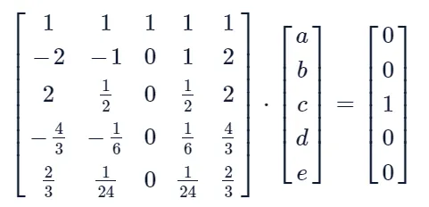
a+b+c+d+e=0

-2a-b+d+2e=0

2a+b/2+d/2+2e=1

-4a/3-b/6+d/6+4e/3=0

2a/3+b/24+d/24+2e/3=0

Converting above equation into matrix form:-

MATLAB codes:-

close all

clear all

clc

<!-- [if mso]>
<![endif]-->

A = [1 1 1 1 1;-2 -1 0 1 2;2 1/2 0 1/2 2;-4/3 -1/6 0 1/6 4/3;2/3 1/24 0 1/24 2/3];

B = [0;0;1;0;0];

X = linsolve(A,B);

 

Result:-

 

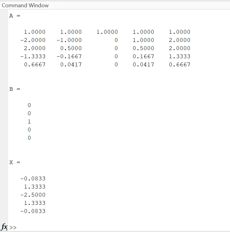
Here, value of a=e and b=d

a=e=-0.0833; b=d=1.3333; c=-2.5000.

2. Skewed Right-Sided Difference Scheme:-
The skewed right-sided difference scheme uses points to the right of the central node for approximation.

Consider the Taylor series expansion of the function f(x) about the point x:

f(x + h) = f(x) + hf'(x) + (h^2/2)f''(x) + (h^3/6)f'''(x) + (h^4/24)f''''(x) + O(h^5)

f(x + 2h) = f(x) + 2hf'(x) + (4h^2/2)f''(x) + (8h^3/6)f'''(x) + (16h^4/24)f''''(x) + O(h^5)

Substituting these expansions into the approximation equation, we get:

f''(x) ≈ (2f(x + h) - 5f(x) + 4f(x - h) - f(x - 2h))/(h^2)

4th order Approximations of 2nd order Derivaive using SKEWED RIGHT-SIDED DIFFERENCING SCHEME:-

Number of nodes = p + q

Hence, number of nodes = 2 + 4  = 6

Taylor's table

Equations:-             

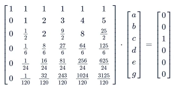
a+b+c+d+e+g=0

0+b+2c+3d+4e+5g=0

0+b/2+4c/2+9d/2+16e/2+25g/2=1

0+b/6+8c/6+27d/6+64e/6+125g/6=0

0+b/24+16c/24+81d/24+256e/24+625g/24=0

0+b/120+32c/120+243d/120+1024e/120+3125g/120=0

Converting above equations into matrix:-

Matlab codes:-

Result:-

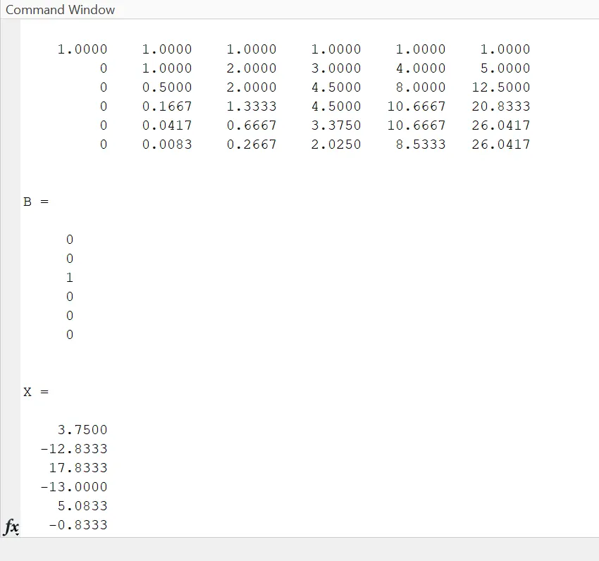
a=3.7500; b=−12.8333; c=17.8333; d=−13.0000; e=5.0833; g=−0.8333.

3. Skewed Left-Sided Difference Scheme:-
The skewed left-sided difference scheme uses points to the left of the central node for approximation. Let's consider the Taylor series expansion of the function f(x) about the point x:

f(x - h) = f(x) - hf'(x) + (h^2/2)f''(x) - (h^3/6)f'''(x) + (h^4/24)f''''(x) + O(h^5)

f(x - 2h) = f(x) - 2hf'(x) + (4h^2/2)f''(x) - (8h^3/6)f'''(x) + (16h^4/24)f''''(x) + O(h^5)

Substituting these expansions into the approximation equation, we get:

f''(x) ≈ (2f(x - h) - 5f(x) + 4f(x + h) - f(x + 2h))/(h^2)

Number of nodes = p + q 

Hence, Number of nodes= 2 + 4  = 6

Taylor's table:-

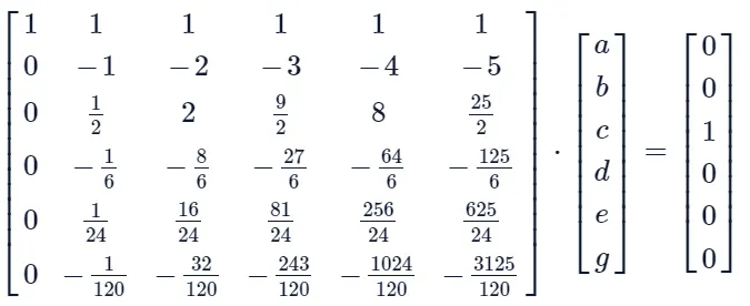
Equations:-            

a+b+c+d+e+g=0

0−b−2c−3d−4e−5g=0

0+b/2+4c/2+9d/2+16e/2+25g/2=1

0−b/6−8c/6−27d/6−64e/6−125g/6=0

0+b/24+16c/24+81d/24+256e/24+625g/24=0

0−b/120−32c/120−243d/120−1024e/120−3125g/120=0

Converting above equations into matrix:-

Matlab codes:-

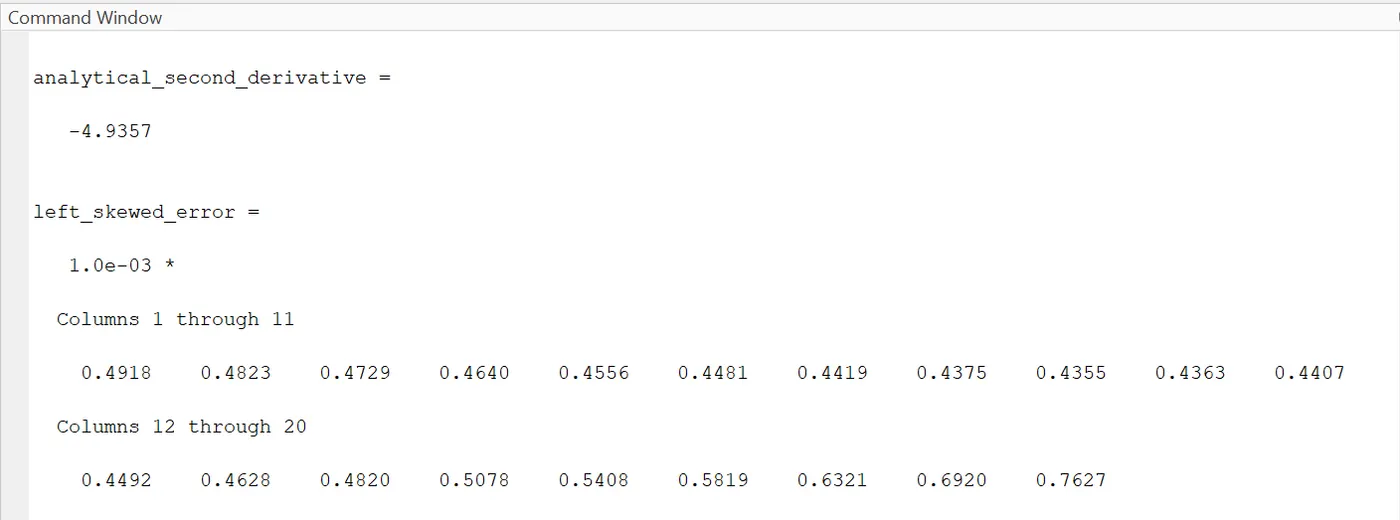
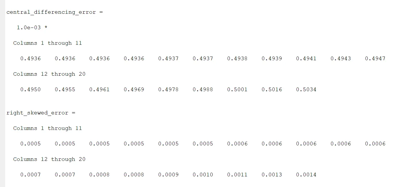
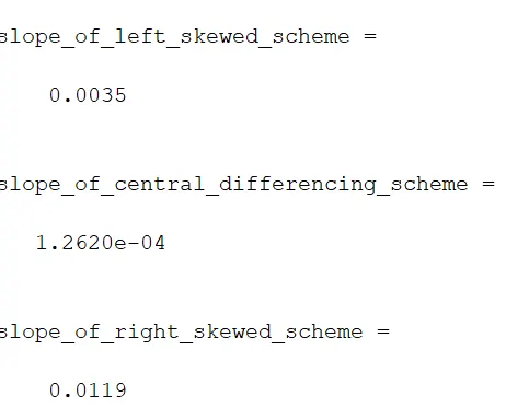
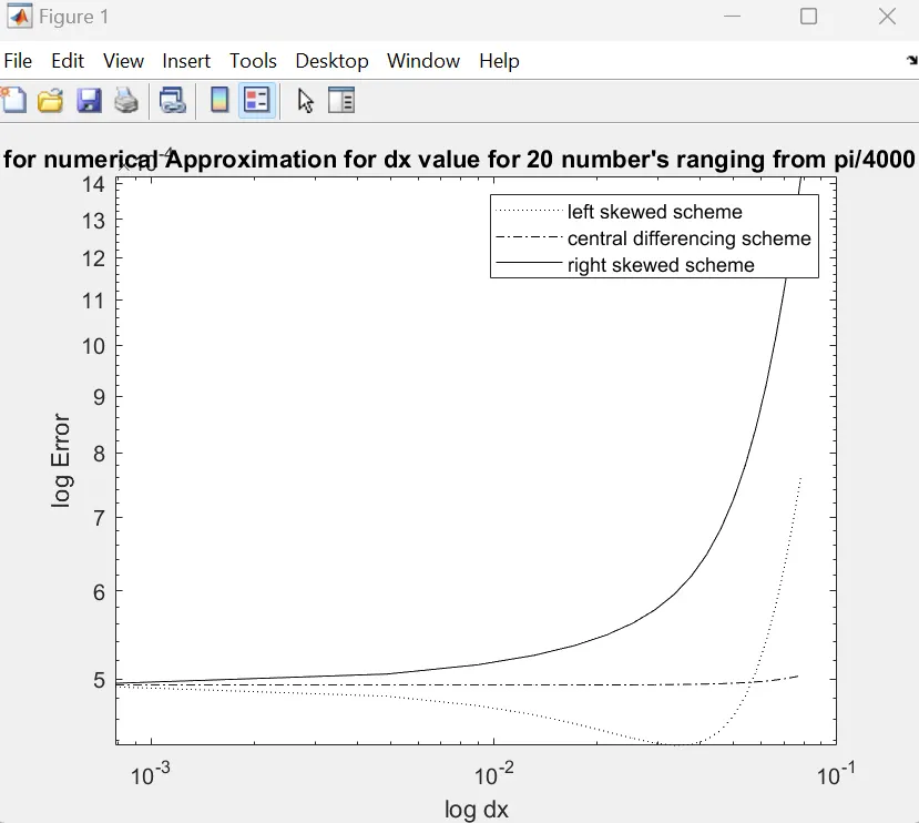
Skewed scheme:-

A skewed scheme is useful because it allows for the approximation of derivatives using points that are not symmetrically located around the central node. This flexibility provides some advantages over the central difference scheme. Here are a few reasons why a skewed scheme can be beneficial:

1. Asymmetric point distribution:- Skewed schemes allow the use of points that are unevenly distributed on one side of the central node. This can be advantageous when dealing with irregular or skewed grids or when specific features of the problem are more pronounced on one side.

2. Local refinement:- In some scenarios, it may be desirable to have a higher resolution or more accurate approximation on one side of the central node compared to the other side. Skewed schemes provide the ability to allocate more points and refine the approximation locally, enhancing accuracy in specific regions of interest.

3. Handling boundary conditions:- Skewed schemes can be useful when dealing with boundary conditions that are better approximated by points located on one side of the central node. For example, when dealing with a boundary where the derivative is known or specified on one side, a skewed scheme can provide a more accurate representation.

4. Improved stability:- In certain cases, using a skewed scheme can improve the stability properties of the numerical method. By distributing the points asymmetrically, it is possible to mitigate numerical oscillations or artifacts that may arise with a symmetric central difference scheme.

Overall, a skewed scheme offers more flexibility in the selection and distribution of points, allowing for tailored approximations based on the specific characteristics of the problem at hand. It provides a way to address asymmetry, local refinement, boundary conditions, and stability concerns that may not be adequately handled by a symmetric central difference scheme.