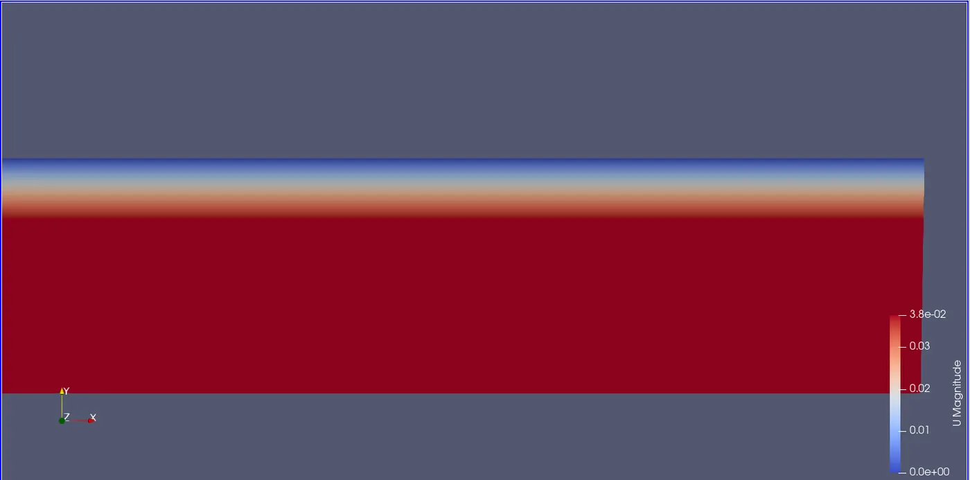
Week 11 - Simulation of Flow through a pipe in OpenFoam
The aim of the project is to simulate wedge shaped section of a pipe. Here we have considered the fluid to be incompressible and the flow to be laminar with Reynolds number as 2100.
Fluid velocity inside the pipe changes from zero (at the surface) due to no-slip boundary condition to maximum (at the centre of the pipe).
Reynolds number:-
The Reynolds number, often denoted as Re, is a dimensionless number used in fluid mechanics to characterize the flow of a fluid (liquid or gas) in a conduit or around an object.
The Reynolds number is defined as:-
Re = (ρ * V * L) / μ
here:
- Re is the Reynolds number.
- ρ (rho) is the density of the fluid.
- V is the velocity of the fluid relative to the object or through the conduit.
- L is a characteristic length or dimension of the object or conduit (e.g., diameter for a pipe or chord length for an airfoil).
- μ (mu) is the dynamic viscosity of the fluid.
Dynamic viscosity:-
Dynamic viscosity, often denoted as μ (mu), is a measure of a fluid's resistance to shear or deformation when subjected to an applied force or stress. In simpler terms, it quantifies how "thick" or "sticky" a fluid is. Dynamic viscosity is a fundamental property of fluids and is an important parameter in fluid mechanics.
Measured in units of pascal-seconds (Pa·s).
The dynamic viscosity of a fluid determines how easily adjacent layers of fluid slide past each other. Fluids with high dynamic viscosity (e.g., honey) are more resistant to flow and exhibit slow, thick, and sticky behavior. In contrast, fluids with low dynamic viscosity (e.g., water or air) flow more easily and have a thinner, less viscous consistency.
Applications:
1. Fluid flow analysis
2. Lubrication
3. Oil and gas industry
4. Pharmaceuticals
5. Food industry
6. Biomedical applications
The Reynolds number is used to predict the type of flow a fluid will exhibit under certain conditions. It helps classify flows into three main categories:
1. Laminar Flow (Re < 2000>) In this regime, the fluid flows smoothly in well-defined layers or streams, with minimal turbulence. The flow is generally predictable, and fluid particles move in parallel paths.
2. Transitional Flow (2000 < Re>) This is a transitional region between laminar and turbulent flow. The flow may exhibit intermittent turbulence and become unpredictable.
3. Turbulent Flow (Re > 4000): In this regime, the fluid flows chaotically with a mix of eddies, swirls, and turbulence. The flow is highly unpredictable, and fluid particles move in irregular patterns.
Hydrodynamic entry length:-
The region from the inlet of the pipe to the point where the velocity profile is fully developed, that distance is called Hydrodynamic entry region. The flow in this region is called hydrodynamically developed flow.
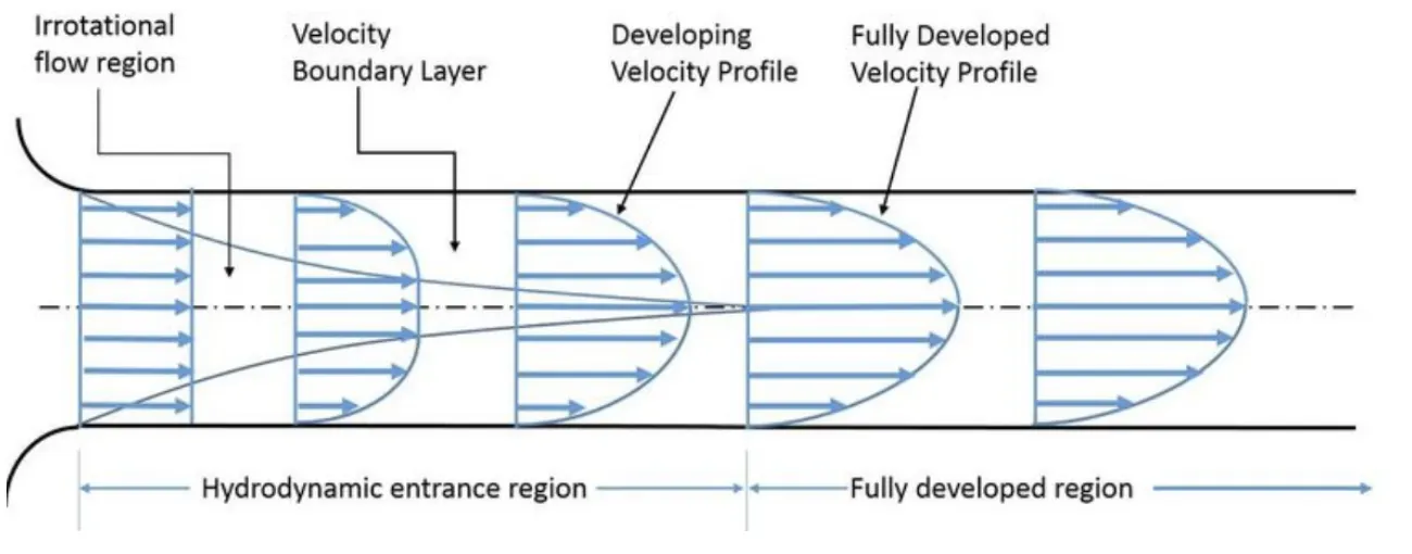
Source:-https://encyclopedia.pub/entry/29470
Hagen-Poiseuille´s equation:-
It is used to calculate headloss (pressure loss) throught circular pipe having laminar flow condition.
The Hagen-Poiseuille equation, also known as Poiseuille's law, describes the flow of an incompressible and Newtonian fluid through a cylindrical pipe or tube.
It provides a mathematical relationship between the flow rate, pressure gradient, viscosity, and geometry of the pipe.
Equation:-
Q = (Π * ΔP * r^4) / (8 * μ * L)
here:
- Q is the volumetric flow rate of the fluid (in cubic meters per second, m⊃3;/s) through the pipe.
- ΔP is the pressure drop along the length of the pipe (in pascals, Pa).
- r is the radius of the pipe (in meters, m).
- μ (mu) is the dynamic viscosity of the fluid (in pascal-seconds, Pa·s).
- L is the length of the pipe (in meters, m).
- The Hagen-Poiseuille equation is applicable only when the flow in the pipe is laminar.
- It emphasizes the relationship between flow rate and pressure gradient.
- Used in engineering and fluid mechanics to design and analyze systems involving the flow of liquids, such as pipelines, blood flow in vessels, and hydraulic systems.
- Limitations: The Hagen-Poiseuille equation is applicable to simple, idealized situations with cylindrical pipes and laminar flow. It doesn't account for complex flow patterns, turbulent flow, or non-Newtonian fluids.
Given:-
- Reynolds number, Re = 2100.
- Length of the entry, Lentry = 0.06*Re*d.
- Diameter of pipe, d = 0.01m.
- Angle of wedge, Theta = 4°.
- Viscosity of water, μ = 0.89e-3 Pa·s
- Density of water, ρ = 997 kg/m⊃3;.
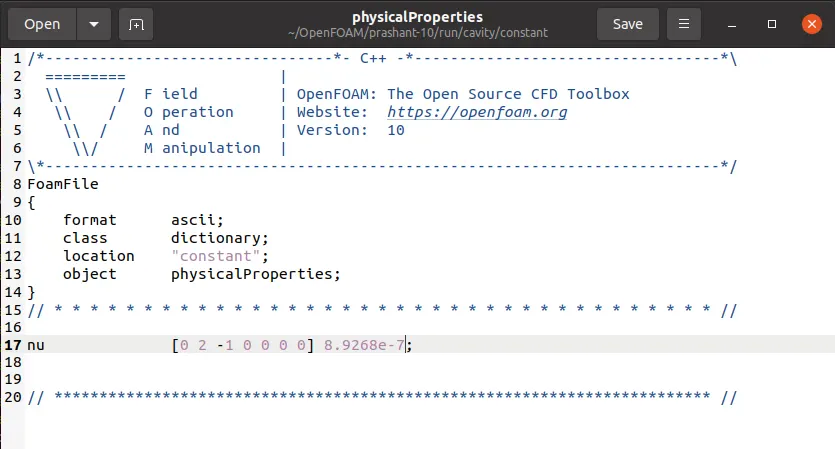
- Kinametic viscosity of water = μ/ρ
- Length of the wedge, L = Lentry + 0.74
- Average velocity, vavg = (Re*μ)/(d*ρ)
- Max velocity, vmax = 2*vavg
- Pressure drop, ΔP = (32*μ*vavg*L)/(d2)
MATLAB codes:-
This matlab code will generate blockMeshDict file for openFoam and validate the expecected results.
clear all
close all
clc

%input parameters
cell_x = 50;
cell_y = 1;
cell_z = 100;
sg_x = 0.2;
sg_y = 1;
sg_z = 1;
Re = 2100; %Reynolds number
d = 0.05; %Diameter of the pipe
r = d/2; %pipe's radius
L_entry = 0.06*Re*d; %length of the pipe
fprintf('Enter 5, 4, 3, 6 for the wedge boundary condition');
theta = 4; %Angle of wedge
mue = 0.89e-3; %viscosity of water at 25°C
rho = 997; �nsity of water at 25°C
nue = mue/rho; %Kinematic viscosity of water at 25°C


�lculating the pressure and velocity
L = L_entry + 0.7; %length of the wedge
v_avg = (Re*mue)/(d+rho); %Average vecocity
v_max = 2*v_avg; %Maximum velocity
del_P = (32*mue*v_avg*0.5)/(d^2); %Pressure drop
kin_P = del_P/rho; %Kinematic pressure drop

%%Validate the fully developed flow velocity profile with its analytical profile
m = csvread("part3.csv",1,0)
v_num = m(:,2)
R = m(:,1)
v_ana = 2*v_avg*(1-((R.^2)/(r.^2)));  %I have interchanged r to R; now r is R and R is r
plot(R,v_ana,':',R,v_num, '*','Color','r')
title("Validated fully developed flow velocity profile with analytical profile")
xlabel("Time (sec)")
ylabel("Velocity (m/s)")
legend("Analytical","Simulated")


�lculating wedge vertices
v0 = [0 0 0];
v1 = [0 r*cosd(theta/2) -r*sind(theta/2)];
v2 = [0 r*cosd(theta/2) r*sind(theta/2)];
v3 = [L 0 0 ];
v4 = [L r*cosd(theta/2) -r*sind(theta/2)];
v5 = [L r*cosd(theta/2) r*sind(theta/2)];

%%BlockMeshDict file
f = fopen('blockMeshDict','w+');
fprintf(f,"/*--------------------------------*- C++ -*----------------------------------*\\\n")
fprintf(f,"  =========                 |                                                  \n")
fprintf(f,"  \\      /  F ield         | OpenFOAM: The Open Source CFD Toolbox            \n")
fprintf(f,"   \\    /   O peration     | Website:  https://openfoam.org                   \n")
fprintf(f,"    \\  /    A nd           | Version:  6                                      \n")
fprintf(f,"     \\/     M anipulation  |                                                  \n")
fprintf(f,"\\*---------------------------------------------------------------------------*//\n")
fprintf(f,"FoamFile\n")
fprintf(f,"{\n")
fprintf(f,"    version     2.0;\n")
fprintf(f,"    format      ascii;\n")
fprintf(f,"    class       dictionary;\n")
fprintf(f,"    object      blockMeshDict;\n")
fprintf(f,"}\n")
fprintf(f,"// * * * * * * * * * * * * * * * * * * * * * * * * * * * * * * * * * * * * * //\n")
fprintf(f," \n")
fprintf(f,"convertToMeters 1;\n")
fprintf(f," vertices\n")
fprintf(f,"(\n")
fprintf(f,"(%d %d %d)\n",v0(1),v0(2),v0(3))
fprintf(f,"(%d %d %d)\n",v1(1),v1(2),v1(3))
fprintf(f,"(%d %d %d)\n",v2(1),v2(2),v2(3))
fprintf(f,"(%d %d %d)\n",v3(1),v3(2),v3(3))
fprintf(f,"(%d %d %d)\n",v4(1),v4(2),v4(3))
fprintf(f,"(%d %d %d)\n",v5(1),v5(2),v5(3))
fprintf(f,");\n")
fprintf(f," \n")
fprintf(f,"blocks\n")
fprintf(f,"(    hex (0 1 2 0 3 4 5 3) (50 1 200) simpleGrading (0.2 1 1)\n",cell_x,cell_y,cell_z)
fprintf(f,");\n")
fprintf(f," \n")
fprintf(f,"edges\n")
fprintf(f,"(\n")
fprintf(f,"    arc 1 2 (0 0.005 0)\n")
fprintf(f,"    arc 4 5 (2.0000 0.005 0)\n")
fprintf(f,");\n")
fprintf(f," \n")
fprintf(f,"boundary\n")
fprintf(f,"(\n")
fprintf(f,"    axis\n")
fprintf(f,"    {\n")
fprintf(f,"        type empty;\n")
fprintf(f,"        faces\n")
fprintf(f,"        (\n")
fprintf(f,"            (0 3 3 0)\n")
fprintf(f,"        );\n")
fprintf(f,"    }\n")
fprintf(f,"    wall\n")
fprintf(f,"    {\n")
fprintf(f,"        type wall;\n")
fprintf(f,"        faces\n")
fprintf(f,"        (\n")
fprintf(f,"            (2 5 4 1)\n")
fprintf(f,"        );\n")
fprintf(f,"    }\n")
fprintf(f,"    inlet\n")
fprintf(f,"    {\n")
fprintf(f,"        type patch;\n")
fprintf(f,"        faces\n")
fprintf(f,"        (\n")
fprintf(f,"            (0 0 2 1)\n")
fprintf(f,"        );\n")
fprintf(f,"    }\n")
fprintf(f,"    outlet\n")
fprintf(f,"    {\n")
fprintf(f,"        type patch;\n")
fprintf(f,"        faces\n")
fprintf(f,"        (\n")
fprintf(f,"            (3 4 5 3)\n")
fprintf(f,"        );\n")
fprintf(f,"    }\n")
fprintf(f,"    wedgeFront\n")
fprintf(f,"    {\n")
fprintf(f,"        type wedge;\n")
fprintf(f,"        faces\n")
fprintf(f,"        (\n")
fprintf(f,"            (0 3 5 2)\n")
fprintf(f,"        );\n")
fprintf(f,"    }\n")
fprintf(f,"    wedgeBack\n")
fprintf(f,"    {\n")
fprintf(f,"        type wedge;\n")
fprintf(f,"        faces\n")
fprintf(f,"        (\n")
fprintf(f,"        (\n")
fprintf(f,"            (0 1 4 3)\n")
fprintf(f,"        );\n")
fprintf(f,"    }\n")
fprintf(f,");\n")
fprintf(f," \n")
fprintf(f,"mergePatchPairs\n")
fprintf(f,"(\n")
fprintf(f,");\n")
fprintf(f," \n")
fprintf(f,"// ************************************************************************* //\n")
%fprintf(f,"\n")
%fprintf(f,"(%d %d %d)",v0(1),v0(2),v0(3))
fclose(f)
Fundamental Units:-
- A fundamental unit is a measurement tool used for a base quantity.
- A fundamental quantity is any physical quantity that cannot be represented in terms of any otherphysical quantity in traditionally defined subset of physical values.
- They are not dependent upon any other units and all other units are derived from them.
- In the SI, fundamental untis are:-
1. Kilograms - Mass
2. Meters - Distance
3. Counting - Seconds
4. Kelvin scale - Temperature
5. Candela of light - Intensity
6. Amperes - Electrical current
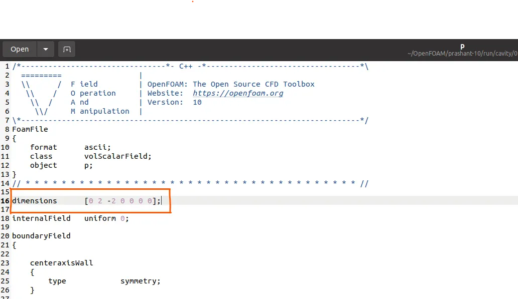
The pressure we have used in this case is in Kinematic Pressure.
Kinematic Pressure:-
Kinematic pressure, often referred to as dynamic pressure, is a concept used in fluid dynamics and aerodynamics to describe a particular type of pressure associated with the motion of a fluid. It is different from static pressure, which is the pressure exerted by a fluid at rest.
Kinematic pressure is defined as:
Kinematic Pressure = 0.5 * ρ * V^2
here:
- Kinematic Pressure is the dynamic pressure.
- ρ (rho) is the density of the fluid.
- V is the velocity of the fluid.
The dynamic pressure is so named because it represents the pressure created by the dynamic motion of the fluid. In other words, it is the pressure due to the kinetic energy of the fluid particles as they move. When fluid flows around an object, such as an aircraft wing or the hull of a ship, the dynamic pressure can vary at different points within the flow. It is an essential parameter in aerodynamics and fluid mechanics for analyzing and designing objects that interact with moving fluids, as it is a key component in equations like Bernoulli's principle and the Euler equations for fluid flow.
In aerodynamics, dynamic pressure is often used to describe the impact of airspeed on an aircraft. Higher airspeed results in higher dynamic pressure, which can affect lift, drag, and other aerodynamic forces on the aircraft. Understanding and controlling dynamic pressure is crucial for the design and operation of various vehicles and structures that move through or interact with fluids.
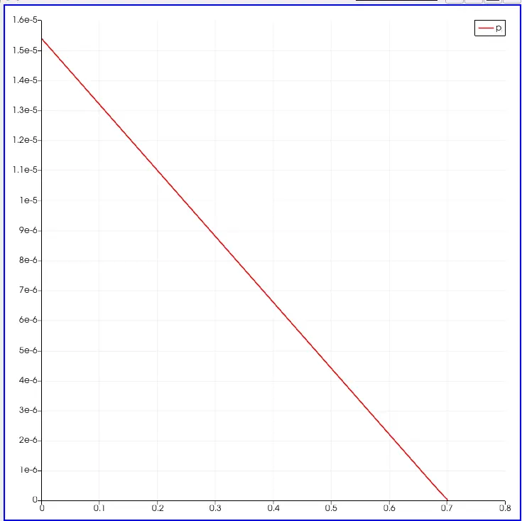
From the graph above plotted, the kinematic pressure is approximately 0.015 and we obtained 0.010 Pascal.
Post-process shear stress:-
- Enable the common toolbar under View -> Toolbars -> Commons.
- Click on calculator and rename the array as mag_U.
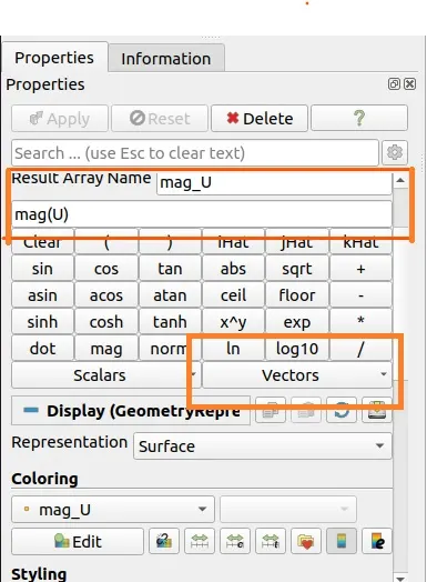
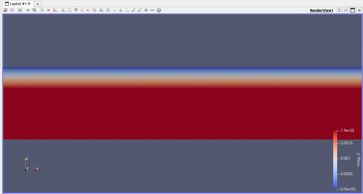
- Now computing the Gradient of magnitude of U by using ctrl + Space.
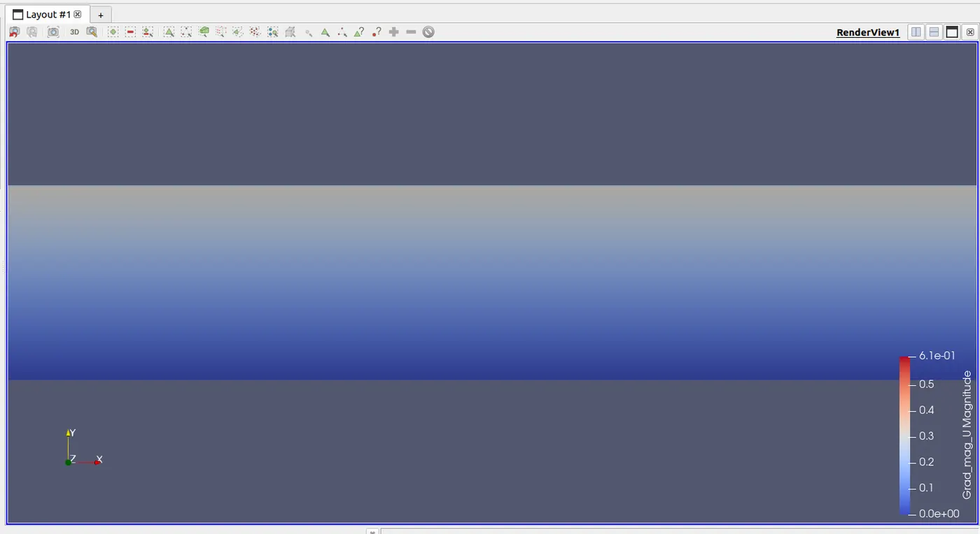
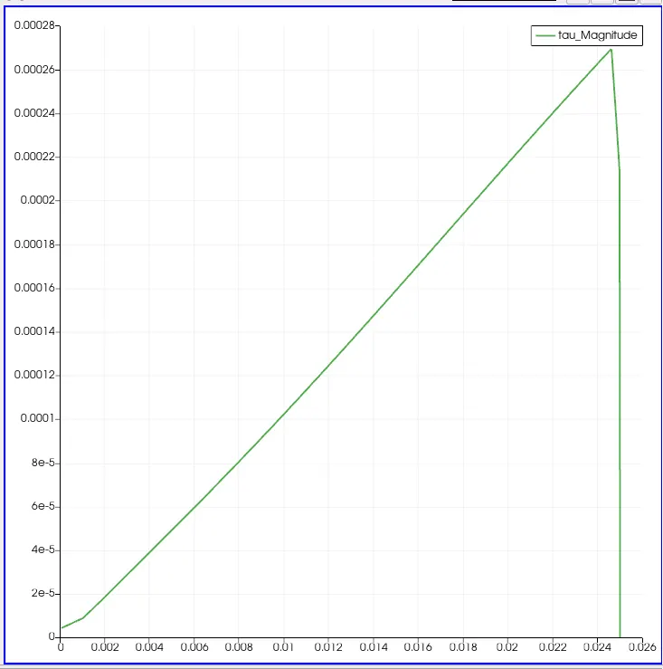
- Now computing magnitude of shear stress from calculator multiplying the grad_mag_U by 0.00089(standard value for water at 25°C) to get shear stress and we get Tau magnitude.
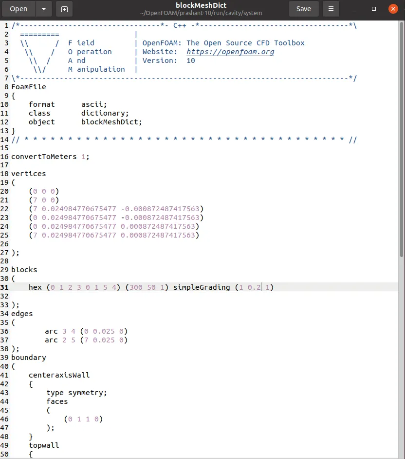
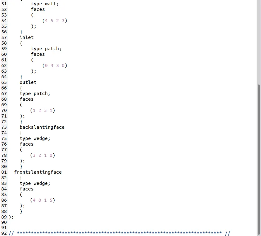
Blockmesh dict file:-
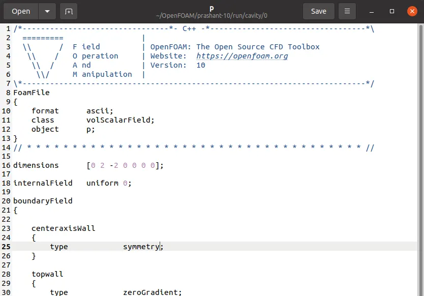
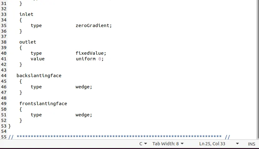
Pressure file:-
Velocity file:-
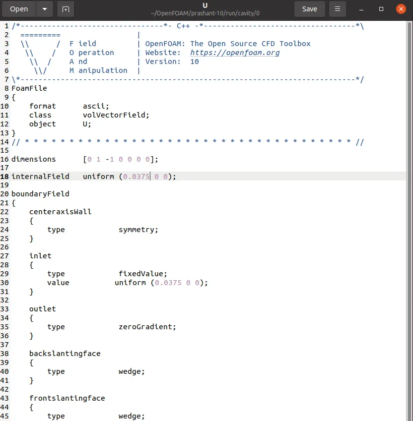
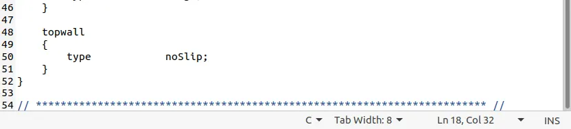
Physical Properties file:-
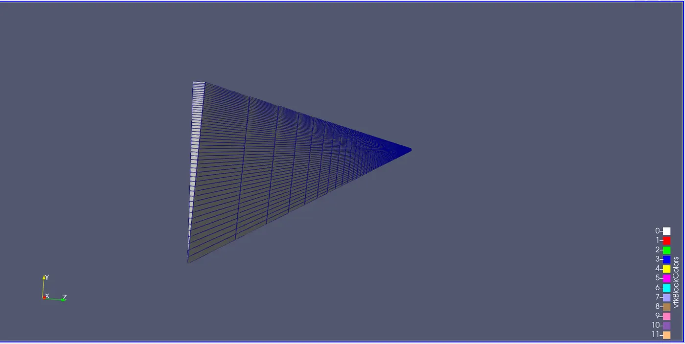
The model and the flow are axis-symmetric along the central line so that all the physical flow have same value and distribution at radius and angle.
Results:-
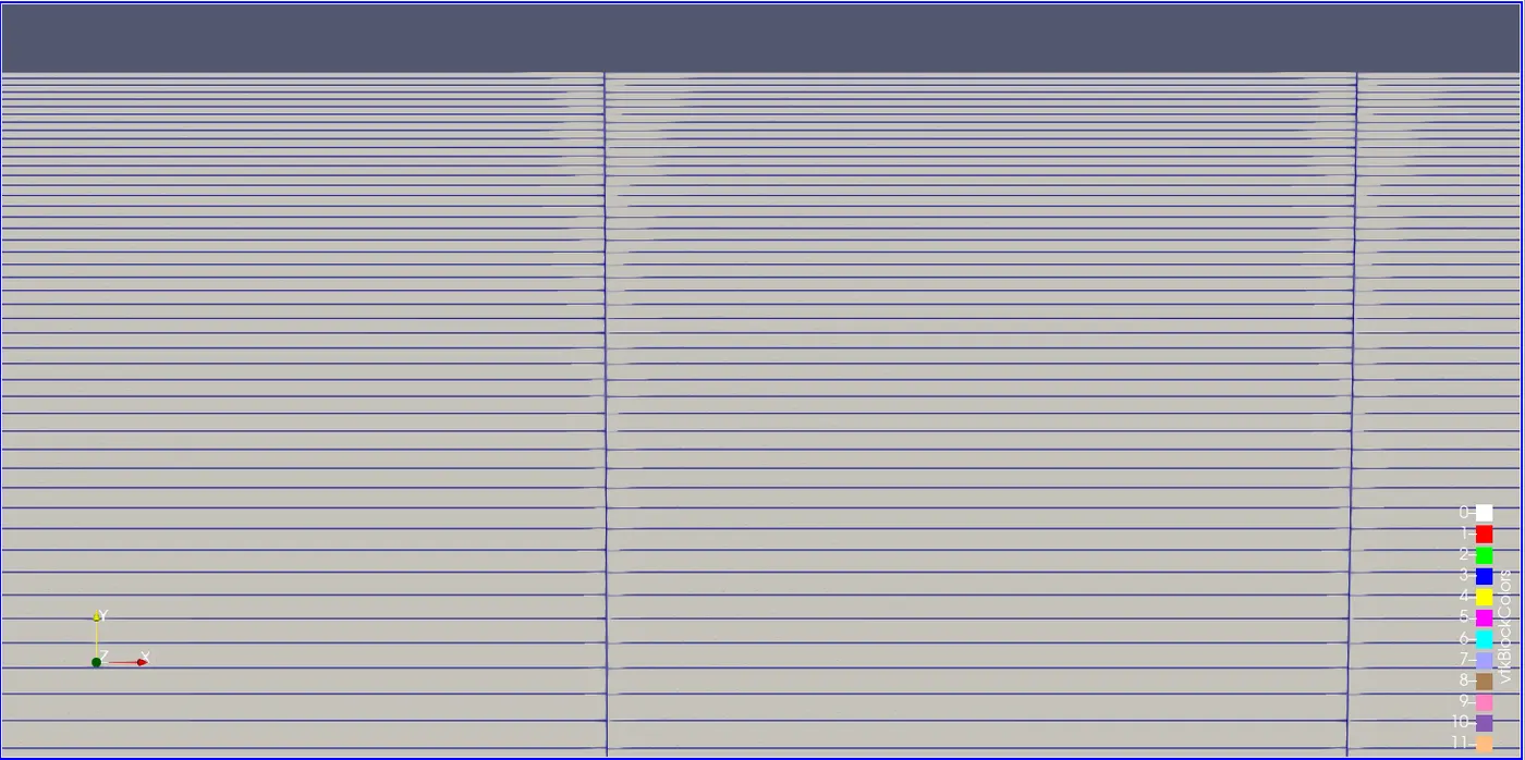
Mesh:-
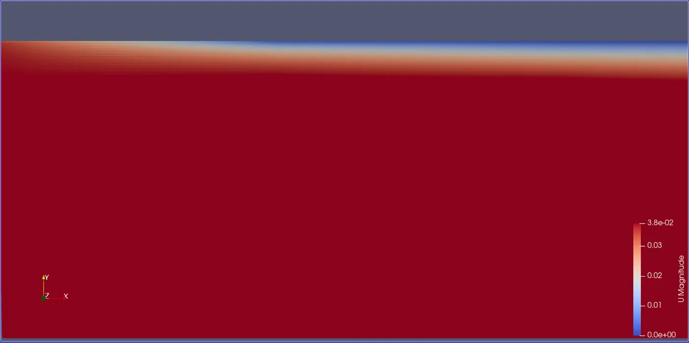
Velocity profile near entrance:-
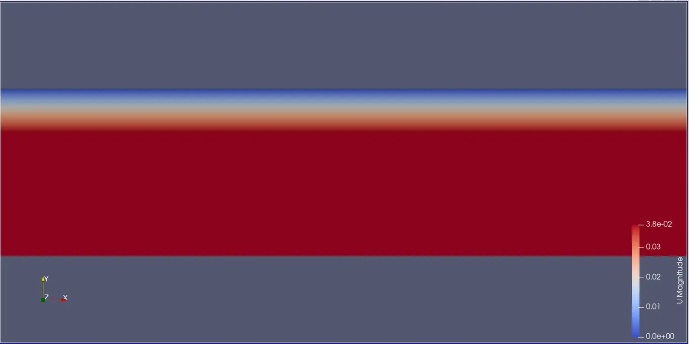
Velocity profile near exit:-