Week 4 - CHT Analysis on Exhaust port

The aim of this assignment is to perform Conjugate Heat Transfer Analysis on an exhaust by appropriately preparing the model’s geometry and then using a base line simulation set up first and then using these results to get a more accurate, convergent solution for the temperature distribution along the walls of the exhaust port from a more refined mesh.

Conjugate Heat Transfer Analysis and it’s uses in Industry and everyday engineering:

Conjugate Heat transfer Analysis is a kind of heat transfer analysis that is done between a fluid and solid. Thus, the computational domain is split into two regions: the fluid domain and the solid domain. The fluid domain is solved for three fields; the pressure, temperature and the velocity using the 3D Navier-Stokes equation. The solid domain is only solved for the temperature using the energy equation. Thus, it simulates the heat transfer between the fluid and the solid domain by exchanging thermal energy at the shared interface.

It has become important in studying the combined effects of thermal conduction in solids and convection in fluids. As this is an important method of heat transfer study, it is broadly used in thermal engineering. It has been widely used to model and simulate natural phenomena and engineering systems and devices such as heat exchangers. CHT is used in aerospace applications, nuclear reactors, thermal goods treatment, medicine, etc.

Geometry set-up (common for both the coarser and finer mesh set-up):

The model was opened in SpaceClaim.

Using the ‘Volume Extract’ option in the ‘Prepare' tab and then selecting the edges of the inlets and the outlets, the inner volume (what is to be the fluid domain) was selected and extracted. This extracted volume was named as ‘Fluid Body’. The solid volume surrounding this extracted volume was named as ‘Solid Body’. A new component was created in the tree and named ‘Final Geometry’. Both the volumes were moved to this newly created component and the empty components were then duly deleted. In the ‘Analysis’ section the ‘Share Topology’ was set to ‘Share’. Since CHT involves the exchanging of thermal energy between the walls, we need a coherent mesh between these two volumes. Thus, in the ‘Workbench’ tab, in the ‘Sharing’ group, the ‘Share’ option was used to generate a common interface.

Meshing (Base line coarse mesh):

A base line mesh was then generated with no forms of refinements.Appropriate named selections were then made.

The inlets and outlets were named as they were. The outer walls of the fluid body were named ‘inflation layers’ and the outer walls of the exhaust were named ‘outer-walls-convection’.

The remaining geometry that is kept unnamed (the solid bodies around the inlets and outlet) will be automatically assigned with the adiabatic boundary conditions.

The adiabatic boundary condition is where the ‘Thermal Conditions’ is set to ‘Heat Flux’ and the value for the heat flux is inputted to be 0 W/m^2.

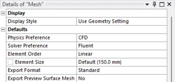
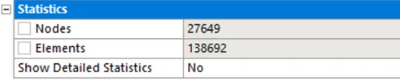
(Mesh details of the base-line mesh.)

Solver Set-Up:

The solver was launched with double precision and 4 processors.

The pressure-based solver was selected (as we can ignore compressibility effects as the Mach number is not high enough).

The energy box was checked. The viscous model chosen was the standard k-epsilon equation.

This is because the yplus would be take in the log-law region.

In the materials section, the fluid domain was taken to be air and solid domain was taken to be aluminium.

Cell boundaries:

Inlet: the velocity was set to 5m/s (magnitude, normal to the boundary). The temperature was set to 700k.

Outer-walls-convection: The thermal conditions was set to Convection and the heat transfer coefficient was inputted to be 20 W*m^-2*k^-1.

The solution was then initialised in the hybrid mode.

Contours of temperature were created for ‘inlets’, ‘outer-walls-convection’, ‘wall-final_geometry-solid_body’.

A report definition was created for wall adjacent heat transfer coefficient.

And an animation was also created for the temperature contour.

This was then solved for 200 iterations.

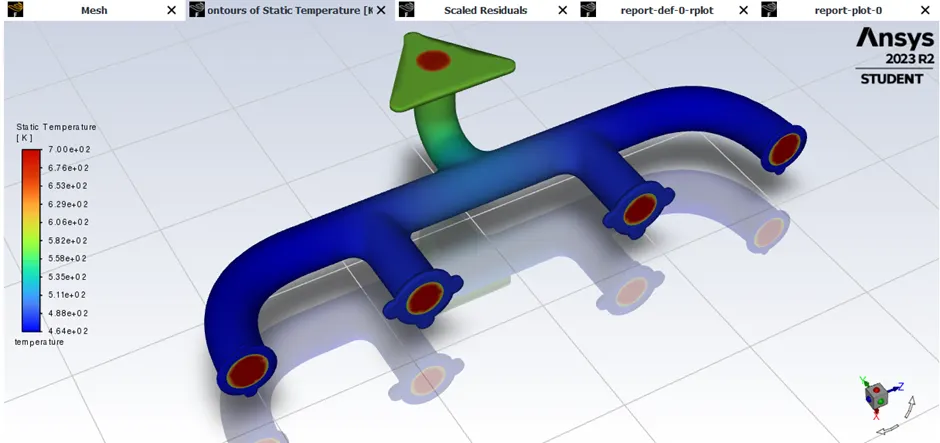
(Temperature contours.)

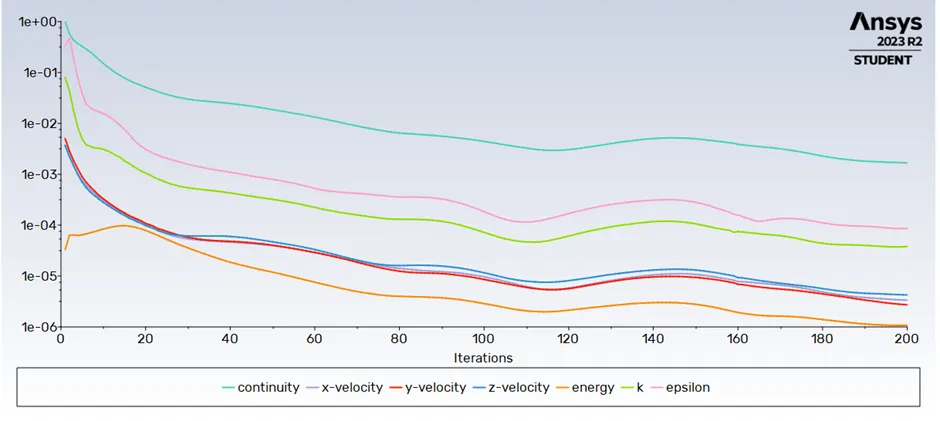
(Scaled Residuals.)

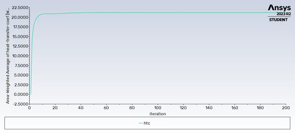
(Area weighted average of heat transfer coefficient.)

The computed value of the HTC is 21.18598.

From the animations we can see that temperature contours show very little changes after 50 iterations or so. Thus, we can say that the solutions have converged. We can safely say that the contours that we get after the calculations are completed is the steady state temperature distribution.

Post processing:

The transparency of the outer walls was set to 80%.

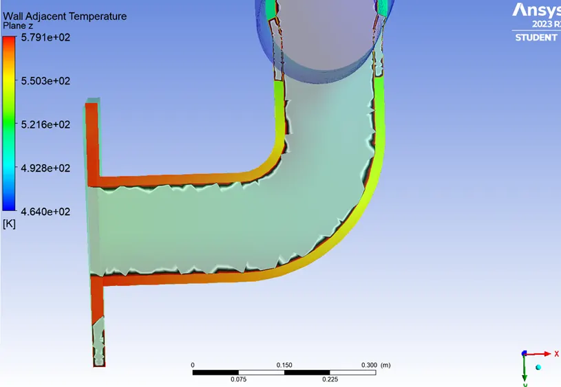
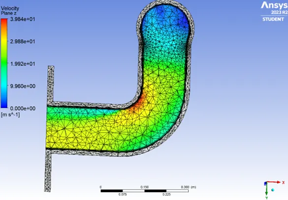
A plane with its normal in the z-direction was created to record the wall adjacent temperature.

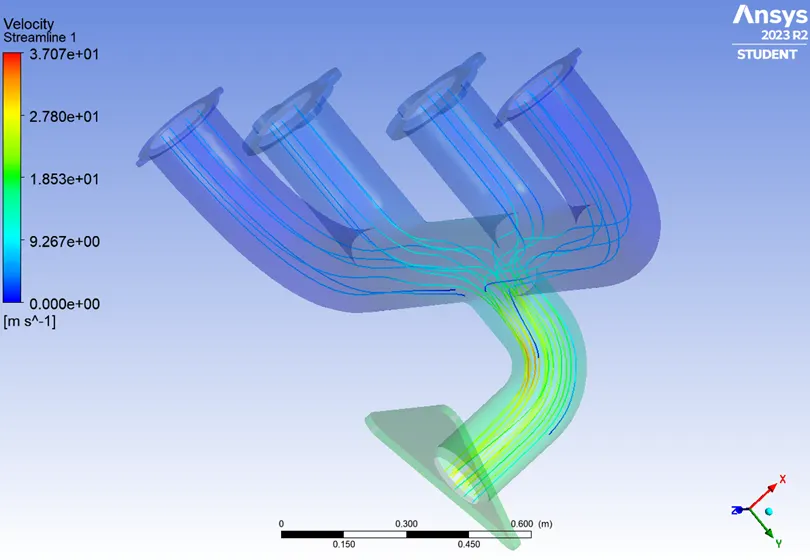
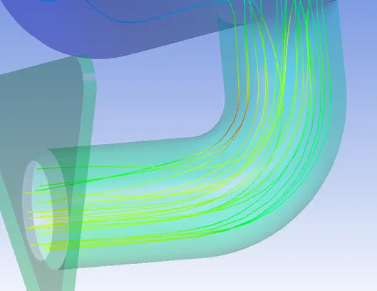
Streamlines were also added that started from the inlet (# of streamlines were set to 25).

Refined set up (with a finer mesh with body-fitted inflation layers):

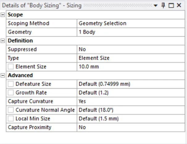
A body sizing was inserted for refining the mesh in the solid body. The mesh length was set to 10mm.The option for ‘Capture Curvature’ was set to ‘Yes’.

For having a body-fitted mesh along the walls to capture the heat flux and the wall adjacent temperature better, inflation layers were inserted at the interface.

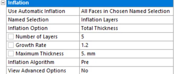
Mesh details and statistics:

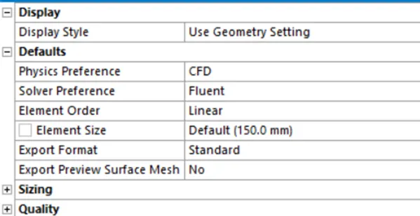
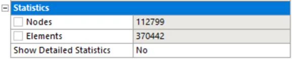
This set up was then initialised (hybrid mode) and then solved for 200 iterations.

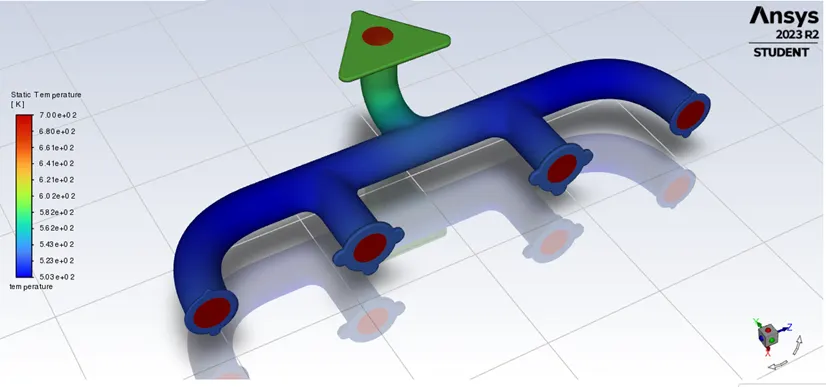
(Temperature contours.)

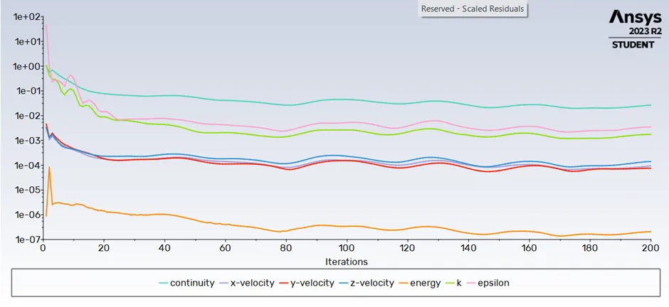
(Scaled Residuals.)

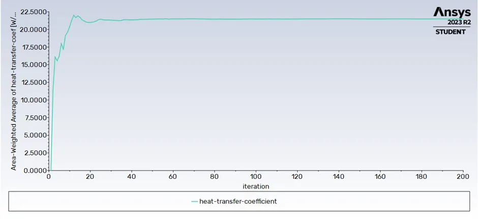
(Area weighted average of heat transfer coefficient.)

The computed value of the HTC is 21.501632.

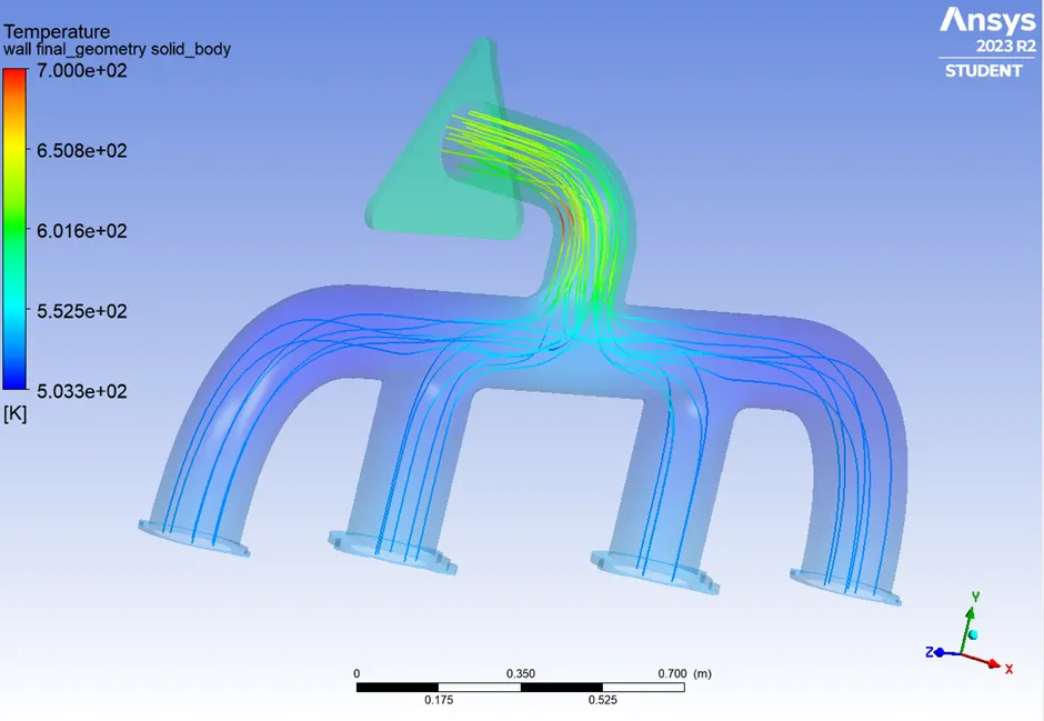
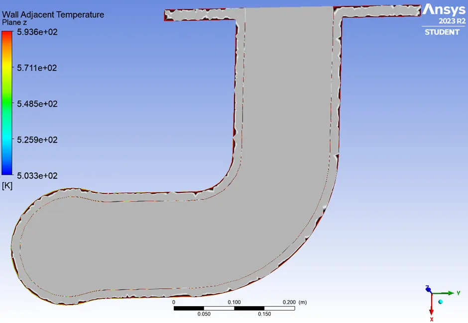
We can say that the results are converging to an accurate value as the temperature contours don’t change significantly after about 50 iterations or so. We can thus say with fair confidence that the solution has converged. We observe a steady state temperature distribution.

Observation and conclusions:

The refined mesh has yielded more sharper and well-defined results.We get more refined solution plots. The body fitted mesh (inflation layers) helps in getting a smooth plot for the wall adjacent temperature.

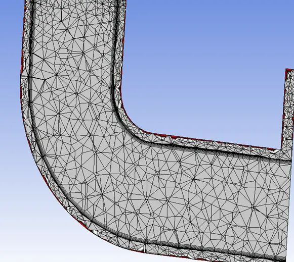
(With the mesh lines.)

We observe that from the velocity streamlines that the flow field show maximum velocity at the bend near the outlet. This is also the region of maximum heat transfer.

How would you verify if the HTC predictions from the simulations are right? On what factors does the accuracy of the prediction depend on?

We observe that from the velocity streamlines that the flow field show maximum velocity at the bend near the outlet. This is also the region of maximum heat transfer. We also know empirically that the bend near the outlet is where the flow field shows maximum velocity and is the region of maximum heat transfer. Thus, this is in conjunction with our results. Another indicator would be that we can find fair correlation between the base-line set up with the coarser mesh and the fine-tuned set-up with finer mesh.

Factors that affect the accuracy of the result.

1)The appropriate kind of solver must be chosen based on the whether we can ignore compressibility effects or not. Here the pressure-based solver was used as mentioned above.

2)Choosing the right viscous turbulence model that is in accordance with the chosen yplus values used while setting up the inflation layer. Here, the data inputted for the inflation layer translates to a yplus in the log-law region. So, in accordance with this, the standard k-epsilon model (a high Re number model) was chosen. If the yplus was less than 5 (viscous sub layer) then the k-omega (a low Re number model) would have been taken.

3)Finer mesh with inflation layers along the walls would definitely yield a more accurate solution.

4)Inputting the right boundary conditions while setting up the solver is of utmost importance for yielding the accurate and convergent solutions.