Week 4 - CHT Analysis on Exhaust port
AIM: CHT Analysis on Exhaust port
OBJECTIVES:
- To give a brief description of why and where a CHT analysis is used.
- To maintain the y+ value according to the turbulence model and justify the results.
- Calculate the wall/surface heat transfer coefficient on the internal solid surface & show the velocity & temperature contours in appropriate areas.
- To verify the HTC predictions from the simulations are right and explain what factors the accuracy of the prediction depends on.
CONJUGATE HEAT TRANSFER
Conjugate heat transfer refers to the coupled analysis of the thermal interactions between fluids and solids. Earlier methods relied on an empirical constant, the heat transfer coefficient, which lumps together all the unknown information regarding the heat transfer process.
Conjugation consists in solving the temperature and heat flux distributions at the fluid-solid interfaces as a coupled problem, without assuming a heat transfer coefficient.
Conjugate heat transfer refers to the coupled analysis of heat transfer between fluids and solids. Heat transfer in fluids occurs through convection, which is a combination of two distinct mechanisms: the microscopic random motion of fluid molecules (diffusion) and the macroscopic bulk fluid motion (advection). In solids, only diffusion is possible (although conduction is the term used to refer to this phenomenon in solids), and it simply amounts to the vibration and collision of particles. Different partial differential equations (PDEs) are used to describe the different physics in the fluids and in the solids. These PDEs are coupled at the fluid-solid interfaces, where the continuity of the temperature and the heat flux must be satisfied.
Application
Conjugate heat transfer is relevant in many engineering applications, where an accurate prediction of the heat transfer and the thermal loading is important. This includes the design of industrial machines and devices, where a proper thermal design has a direct impact on the performance and the lifetime of the devices. Some example applications include:
- <!--[endif]-->Heating, ventilation, air-conditioning (HVAC)
- <!--[endif]-->Cooling of electronic devices
- <!--[endif]-->Heat exchangers
- Gas turbines
- Engine cooling
The stages involved in the simulation are as follows
- <!-- [if !supportLists]-->Geometry
- Mesh
- <!-- [if !supportLists]-->Setup
- <!-- [if !supportLists]-->Solution
- <!-- [if !supportLists]-->Results
Geometry volume extract
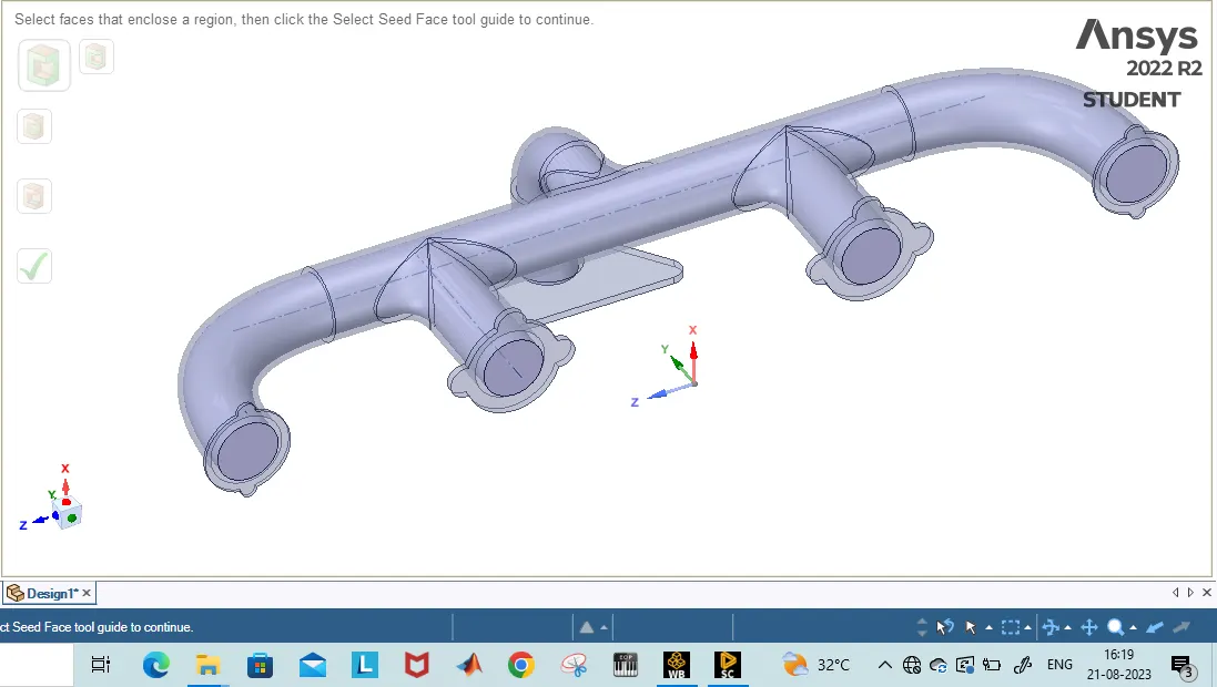
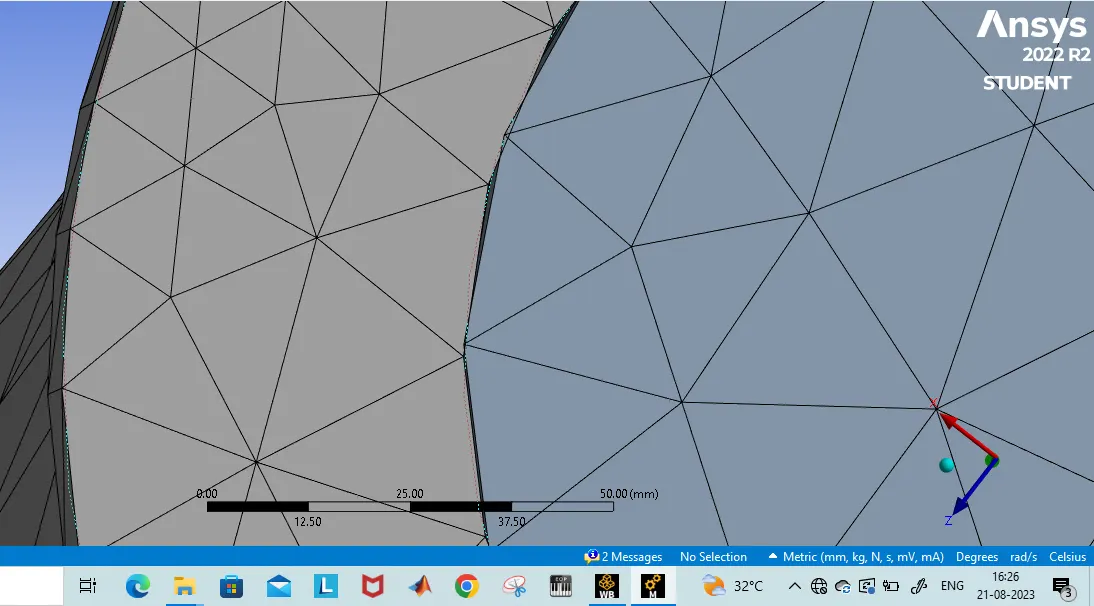
non-conformal meshing formed
exhaust port as single volume
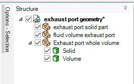
making both volume under the same component
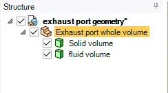
Sharing topology
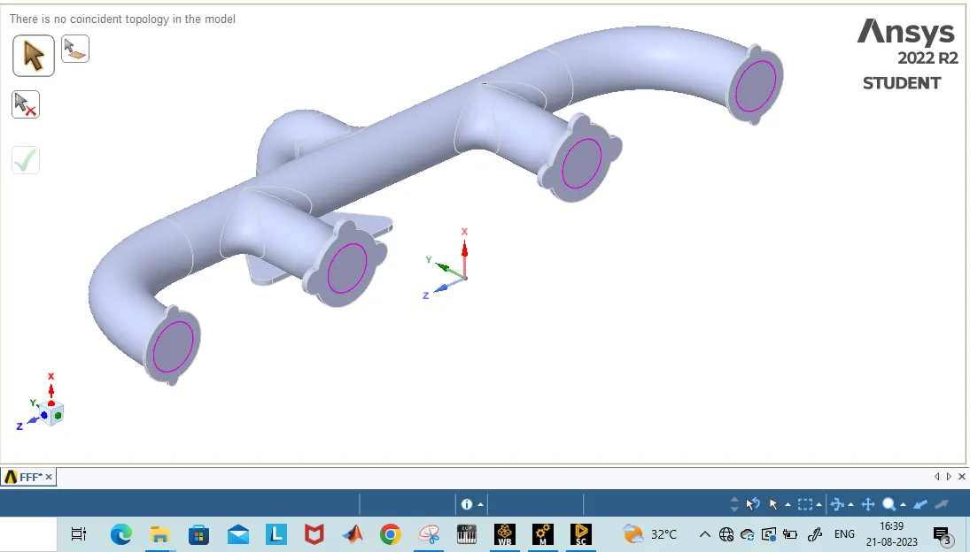
All vertices in fluid and solid parts is coincide with each other
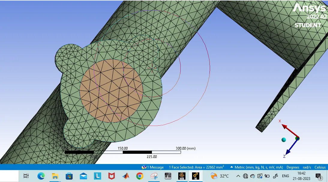
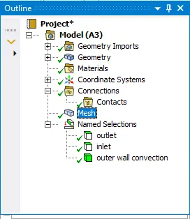
naming is done
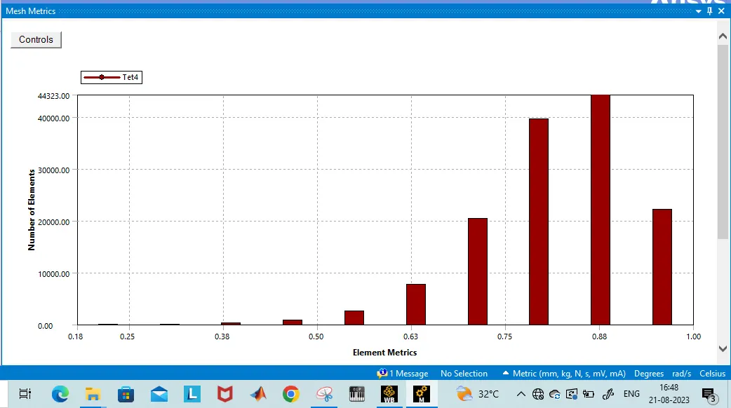
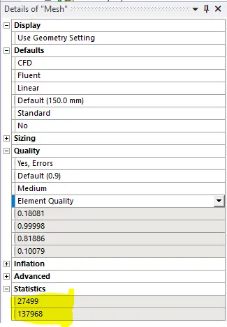
mesh metric greater than 10%
Case 1:
mesh details
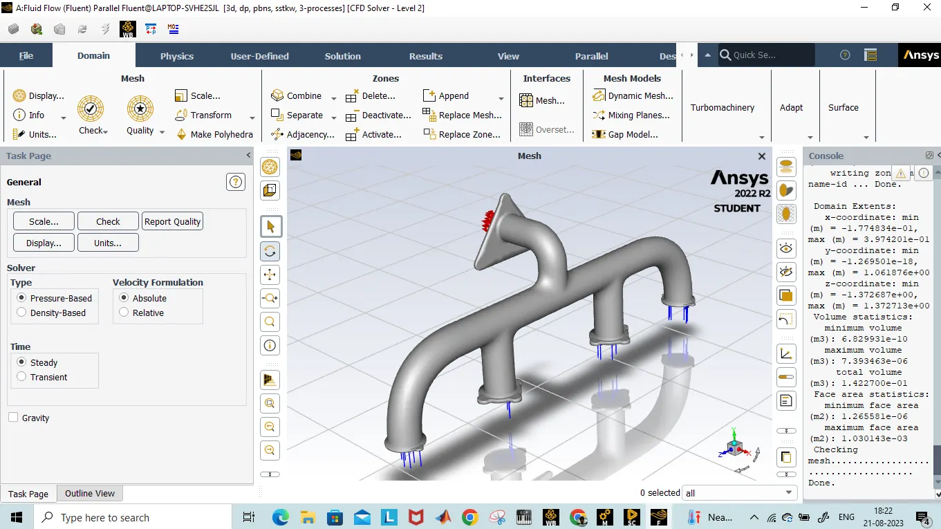
Setting up process
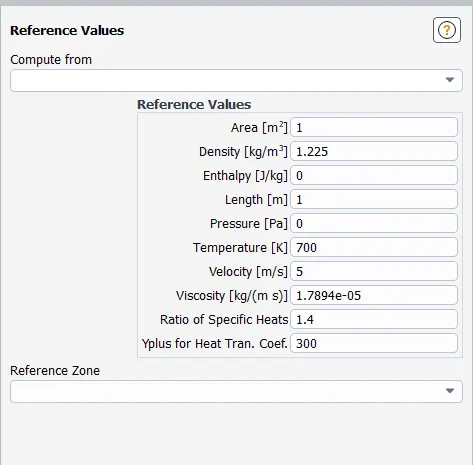
reference values
Solution and Result:
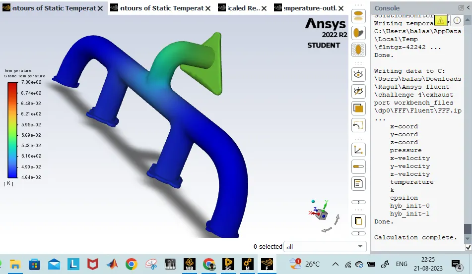
temperature Contour:
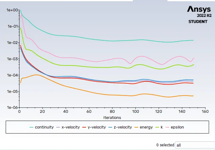
Residuals
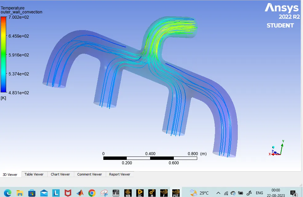
streamline velocity
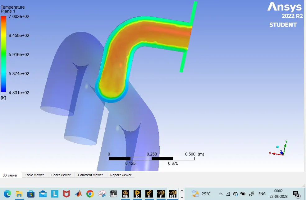
Temperature section plane xy
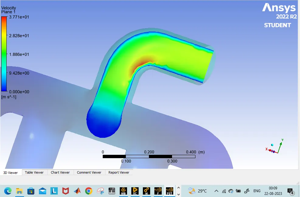
Velocity at section plane
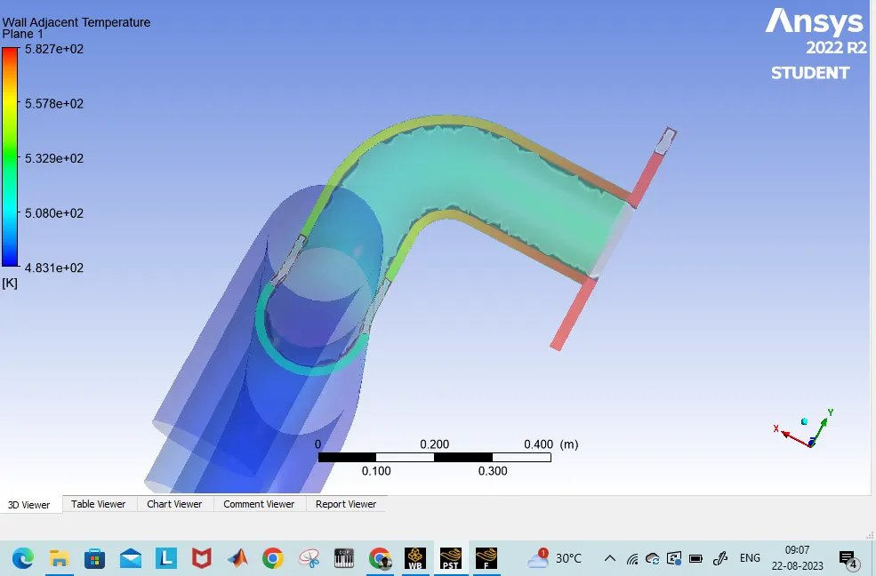
wall adjacent temperature
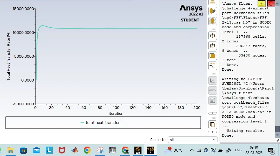
Total heat transfer plot
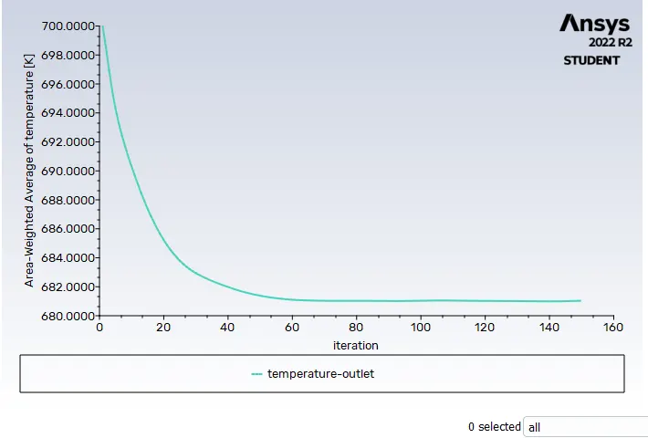
Average temperature outlet as 681°C
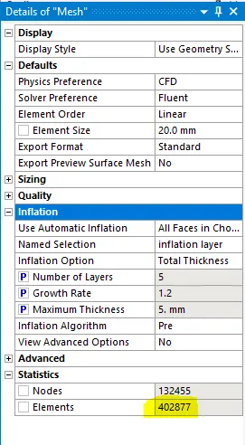
CASE 2:
Mesh Refinement details
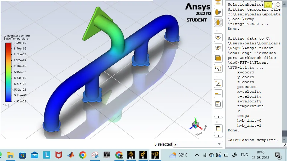
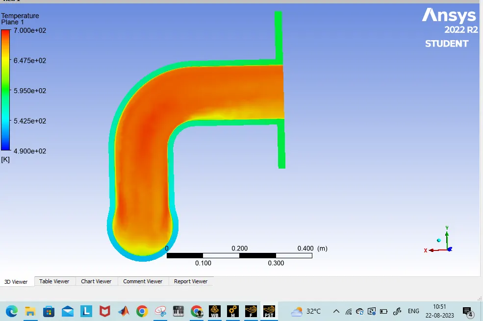
Temperature contour
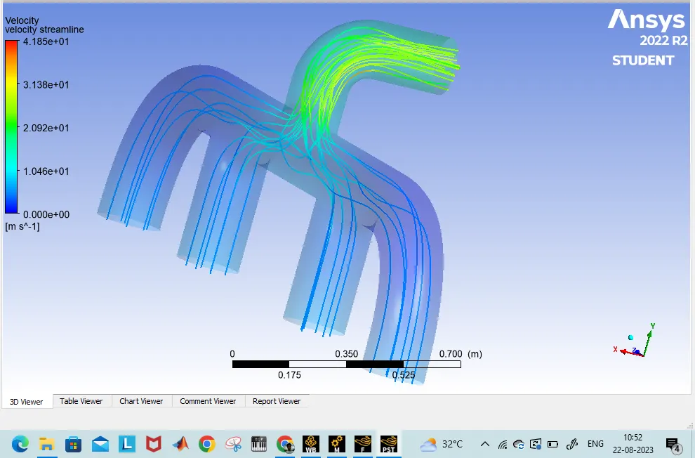
Velocity stream line
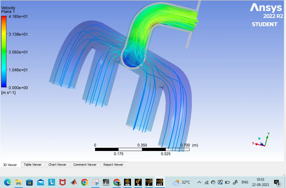
velocity plane with streamline flow
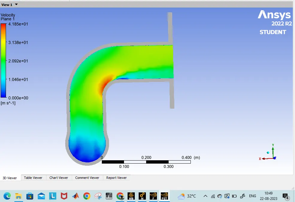
Velocity at section plane
Temperature at section plane
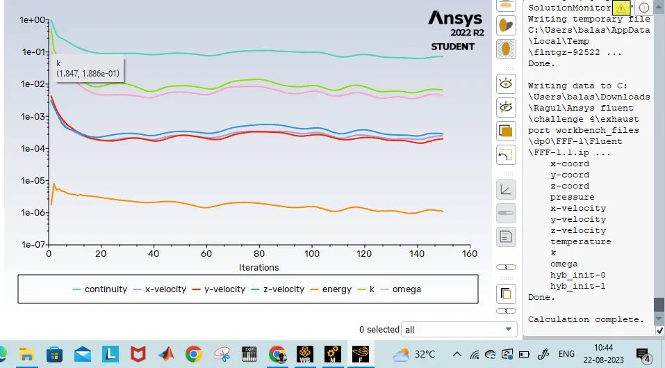
Residuals
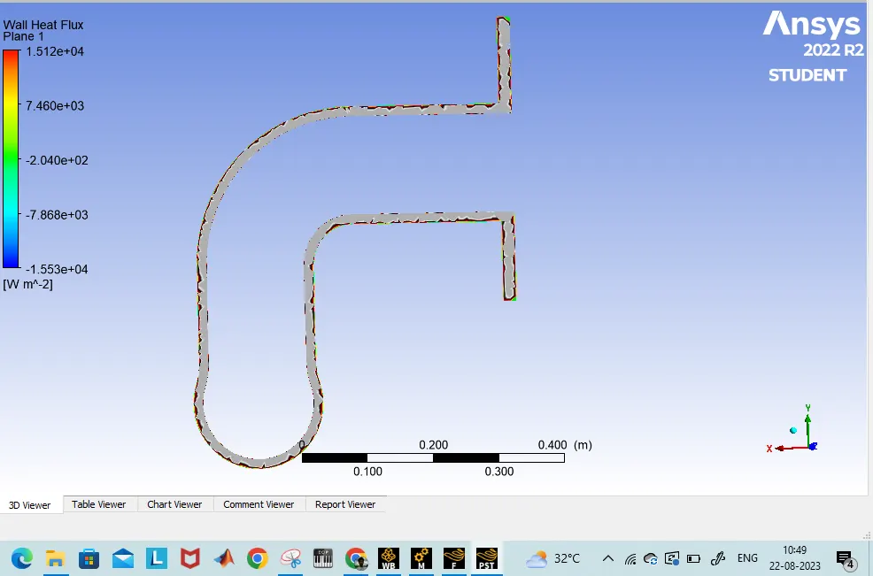
Wall heat flux
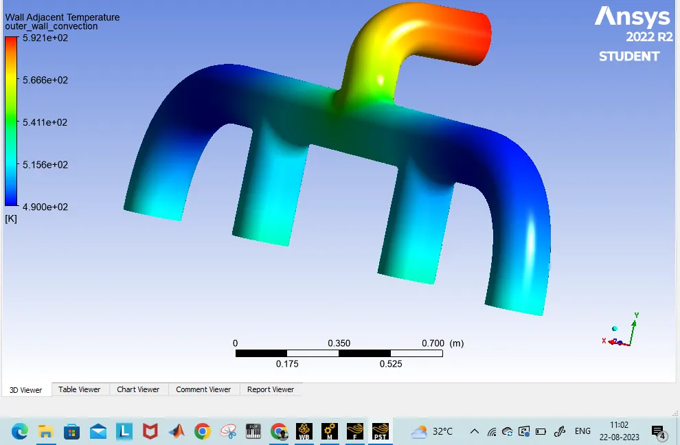
Wall adjacent temperature
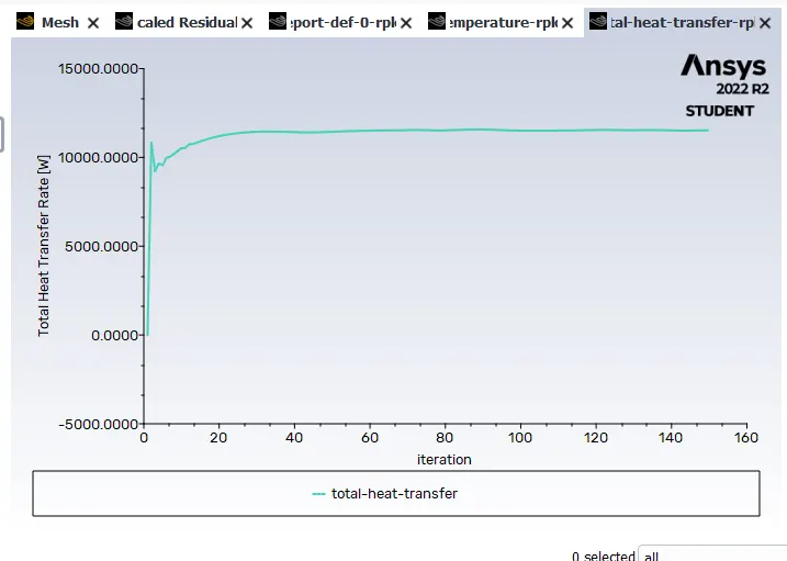
Total heat transfer rate
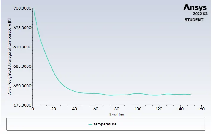
Average temperature outlet as 678°C
Y+ value
The Y+ value is a dimensionless parameter that represents the distance from the first grid cell to the surface wall.
In computational fluid dynamics (CFD), y+ is a dimensionless wall distance used to evaluate the accuracy of turbulence models near solid boundaries. Different turbulence models have different y+ requirements for accurate predictions of the near-wall flow.
For instance, when using the standard k-epsilon turbulence model, it is generally recommended to use a y+ value between 30 and 300 to ensure accurate predictions of the near-wall flow. On the other hand, when using the Reynolds stress model (RSM), a lower y+ value (around 1) is recommended to accurately capture the anisotropy of the turbulence near the wall.
To use y+ values with different turbulence models in CFD, We first need to determine the desired y+ range for the particular turbulence model we are using. We can then adjust the mesh size and/or the near-wall cell size in your CFD simulation to achieve the desired y+ value in the near-wall region.
There are several methods for achieving the desired y+ value, including using the wall function approach, the non-equilibrium wall function approach, or the direct numerical simulation (DNS) approach. The wall function approach is the most commonly used method, and it involves applying a logarithmic law of the wall to the near-wall region to obtain the wall shear stress, which is then used to compute the turbulent viscosity in the rest of the domain.
Different turbulence models have different requirements and guidelines for the appropriate range of y+ values. Here's a general overview of how y+ values are used with different types of turbulence models:
<!-- [if !supportLists]-->1. <!--[endif]-->Spalart-Allmaras (SA) Model: The SA model is widely used for boundary layer flows. For this model, a y+ value between 30 and 300 is recommended. It is typically advised to keep the y+ value below 200 to ensure accurate predictions. Near the wall (y+ < 1> 30), the turbulence model equations are directly solved.
<!-- [if !supportLists]-->2. <!--[endif]-->k-epsilon Models: The k-epsilon models, such as the standard k-epsilon and the RNG k-epsilon, are widely used for a range of applications. For these models, a y+ value between 30 and 200 is typically recommended. In the near-wall region (y+ < 30> 200), the turbulence model equations are directly solved.
<!-- [if !supportLists]-->3. <!--[endif]-->k-omega Models: The k-omega models, including the standard k-omega and the SST k-omega, are commonly used for complex flows. These models require a y+ value between 1 and 5 in the near-wall region. This ensures accurate predictions without using wall functions. In the outer region, the turbulence model equations are directly solved.
<!-- [if !supportLists]-->4. <!--[endif]-->Reynolds Stress Models (RSM): RSMs provide more detailed predictions of turbulence by considering the Reynolds stresses. They are suitable for complex flows. In RSMs, it is recommended to use a low y+ value (< 1>
To ensure accurate results, it is important to ensure that the first cell center is located within the appropriate y+ range for the chosen turbulence model. This can be achieved by adjusting the mesh size and/or using a wall function approach that extrapolates the solution to the wall.
How would you verify if the HTC predictions from the simulations are right? On what factors does the accuracy of the prediction depend on?
Nusselt number is given by:
<!-- [if gte vml 1]>
where:
D is the inside diameter of the circular duct
Pr is the Prandtl number
n=0.4 for the fluid being heated, and n=0.3 for the fluid being cooled.
Nu= Nusselt's Number
Re = Renold's number
It means Nusselt no. is the function of Reynolds no and Prandtl number
As the turbulent boundary layer in the bend of the outlet port is the thin maximum velocity of flow is observed at bend and hence higher Reynolds number.
Now,
Nu=h*L/K
therefore, h=Nu*K/L
where,
- h= Heat Transfer Coefficient
- Nu= Nusselt's Number
- K= Thermal conductivity coefficient
- L= Characteristic Length
As the length of pipe and thermal conductivity is a constant value of h will increase as Nu increases and Nu increases as Re increases.
As per our result, the heat transfer coefficient is high for a higher value of velocity and hence our results are correct.
FACTORS AFFECTING THE QUALITY OF PREDICTION:
- More refined mesh leads to better results
- Use inflation layers and apply boundary conditions
- Proper selection of turbulence model according to Y+ values.