Week 4 - CHT Analysis on Exhaust port

Conjugate heat transfer (CHT):

The Conjugate Heat Transfer (CHT) analysis type allows for the simulation of heat transfer between solid and fluid domains by exchanging thermal energy at the interfaces between them. Typical applications of this analysis type exist as but are not limited to, the simulation of heat exchangers, cooling of electronic equipment, and general-purpose cooling and heating systems.

The modern conjugate convective heat transfer model was created after computers became widely used to replace the heat transfer coefficient, which had been the only tool available for theoretical heat convection since Newton's time, with the empirical relationship of proportionality of heat flux to temperature difference. This model addresses the heat transfer between a body and a fluid running over or inside it as a result of the contact between two objects. It is based on a rigorously mathematically described issue. For each item in two subdomains, the physical operations and governing equation solutions are taken into account individually. The distributions of temperature and heat flux along the body-flow interface are provided by matching conditions for these solutions at the interface, negating the necessity for a heat transfer coefficient.

Using CHT analysis because:

By simultaneously resolves all the pertinent solid and flow field heat transfer processes, such as conduction through solids, free and forced convection in the gases/fluids, thermal radiation, computational fluid dynamics (CFD) and more specifically conjugate heat transfer (CHT) analysis can accurately predict heat transfer. Since wall heat transfer coefficients and their local changes on surfaces are directly estimated within the model rather than relying on reduced empirical estimates, the CHT technique offers an advantage over FE thermal evaluations. Therefore, the CHT technique provides advantages for applications where heat transmission is either non-uniform or challenging to estimate experimentally.

Conjugate Heat Transfer (CHT) is a numerical analysis technique used to study the transfer of heat between fluids and solid structures. It is typically employed in engineering and scientific fields to analyze heat transfer phenomena in systems where both fluid flow and solid conduction are significant.

Here are some common applications where Conjugate Heat Transfer analysis is used:

1. Electronics Cooling: CHT analysis helps in studying the heat transfer in electronic devices such as computer chips, circuit boards, and heat sinks. It allows engineers to optimize cooling strategies to prevent overheating and ensure the reliability of electronic components.
2. Gas Turbines and Aeroengines: CHT analysis is employed to analyze the thermal behavior of gas turbine components, such as turbine blades, combustion chambers, and nozzle guide vanes. It aids in optimizing cooling mechanisms, reducing thermal stresses, and enhancing the overall efficiency of the system.
3. Automotive Industry: CHT analysis is utilized in the design and development of automotive engines, exhaust systems, and cooling systems. It helps engineers understand and optimize heat transfer within the engine components, radiator, exhaust manifold, and other critical parts.
4. Aerospace Applications: In the aerospace industry, CHT analysis is used to investigate the thermal behavior of aircraft components, such as wings, fuselage, and propulsion systems. It enables engineers to evaluate and improve the heat transfer characteristics, thermal stresses, and overall performance of these components
5. Power Generation: CHT analysis plays a crucial role in designing and optimizing thermal power plants, nuclear reactors, and energy systems. It aids in understanding the heat transfer.

Procedure

• Open a new fluent tree in Ansys WorkBench.
• Import the model into geometry.
• The geometry has now been modified to remove any extraneous corner portions. Additionally, extract the volume in the model and name the inner volume as fluid and outer volume as solid volume.

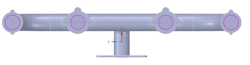
• Once the geometry setup is completed in SpaceClaim, proceed to open the meshing module.
• In the meshing module, select the desired faces on the geometry and assign appropriate names to them for better organization.
• Create a named selection specifically for the fluid volume to facilitate the application of an inflation layer. This step is crucial for the conjugate heat transfer analysis between the fluid volume and the solid wall.
• Implement a body sizing operation on the outer wall's convection region. This approach aims to achieve mesh refinement in critical areas and ensures accurate results are captured in these regions.

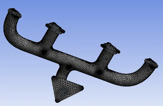
• After updating the mesh in Fluent, open the Fluent setup and select a pressure-based solver with steady-state time simulation and the absolute velocity formulation under the general settings.
• Under the physics menu, choose the energy option since we are dealing with temperature properties.
• Input the boundary values at the inlet: set the inlet velocity to 5 m/s and the inlet temperature to 700K.
• Set the outer wall convection boundary to the convection type and input a constant value of 20 `w/(m^2k)`for the heat transfer coefficient.
• Under the materials properties, select "air" as the fluid material and "aluminum" as the solid material.
• Enter the reference values according to the geometry and inlet boundary conditions. Initialize the simulation using the hybrid initialization method.
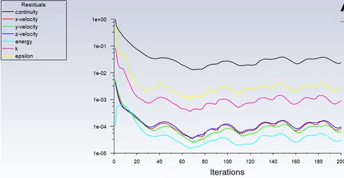
• Run the simulation for certain no of iterations as it is often sufficient to achieve a converged solution.

	Element size	No. of Elements
Case 1	50mm	2.5 lak
Case 2	75mm	3.0 lak
Case 3	100mm	3.5 lak

Results

Contours

CASE 1

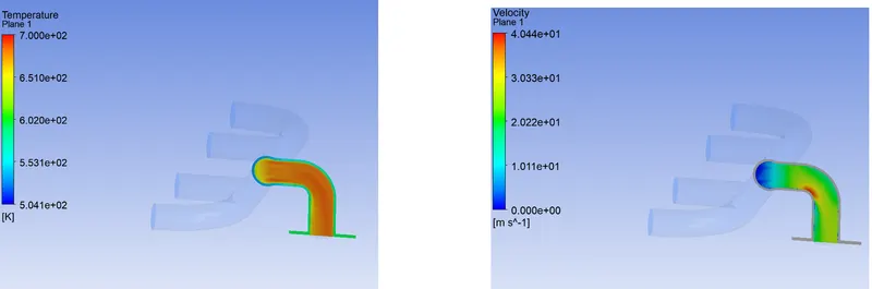
Temparature distribution:

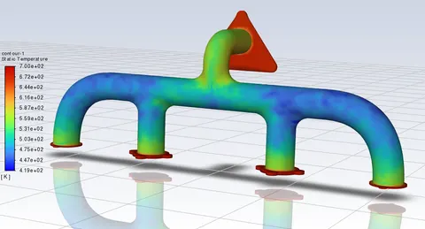
Residual plot

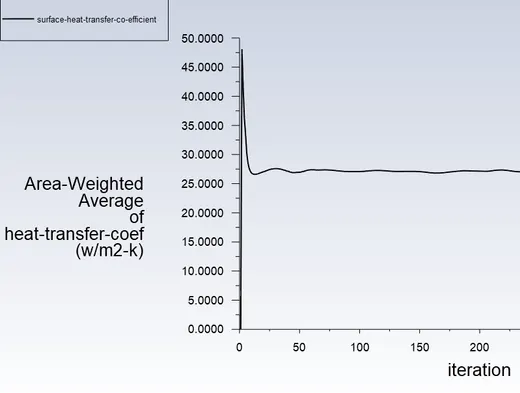
surface heat transfer co-efficient

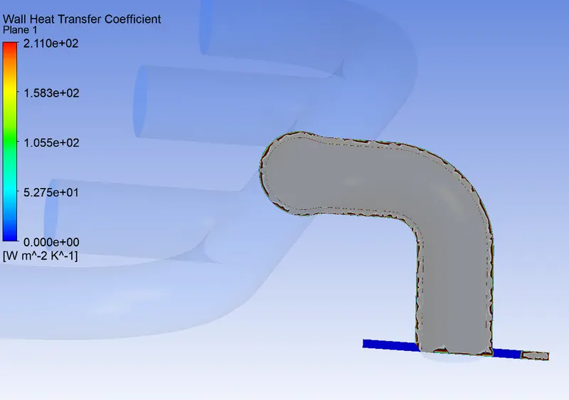
wall heat transfer coefficient

Temperature and velocity contours

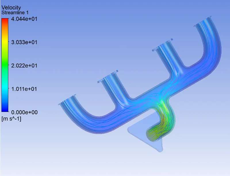
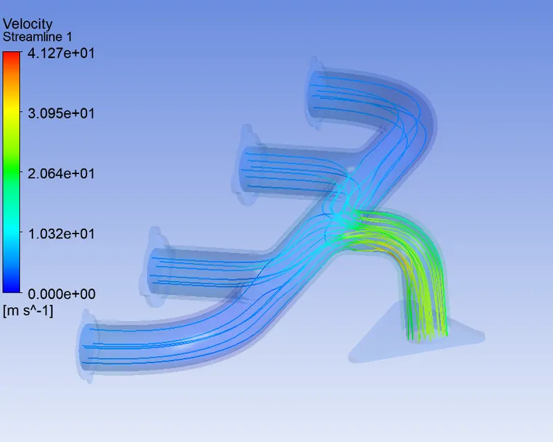
velocity streamlined plot

CASE 2

Temparature distribution:

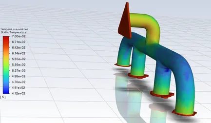
Residual plot:

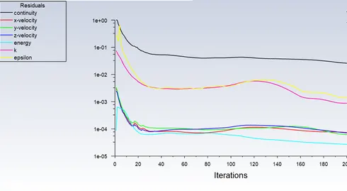
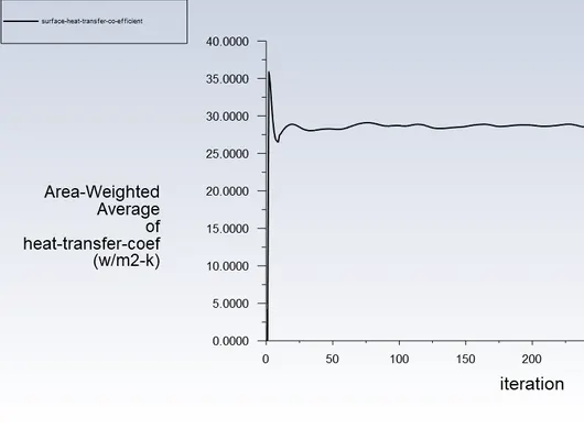
surface heat transfer co-efficient:

Temperature and velocity contours:

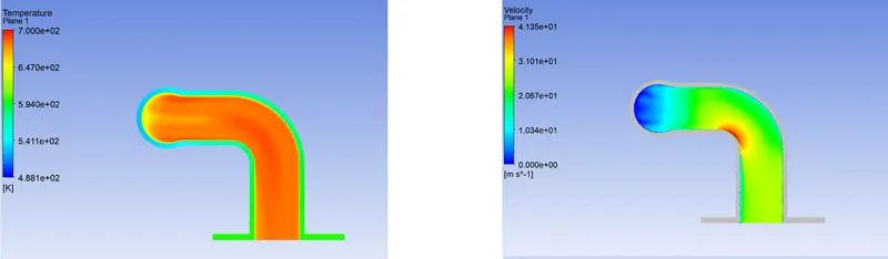
velocity streamlined plot

CASE 3

Temparature distribution:

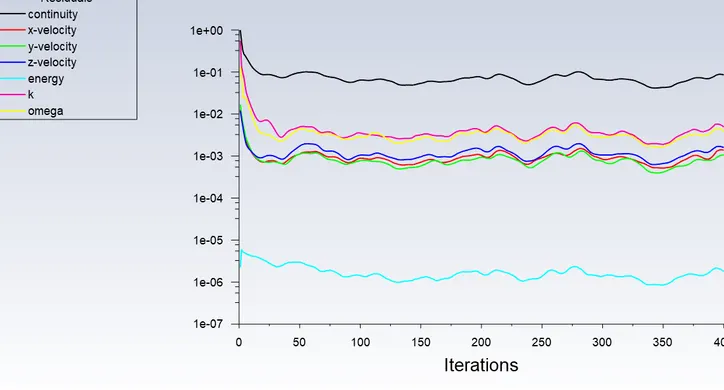
Residual plot

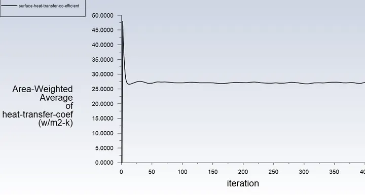
surface heat transfer co-efficient

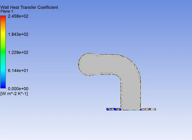
wall heat transfer coefficient

Temperature and velocity contours

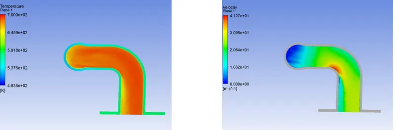
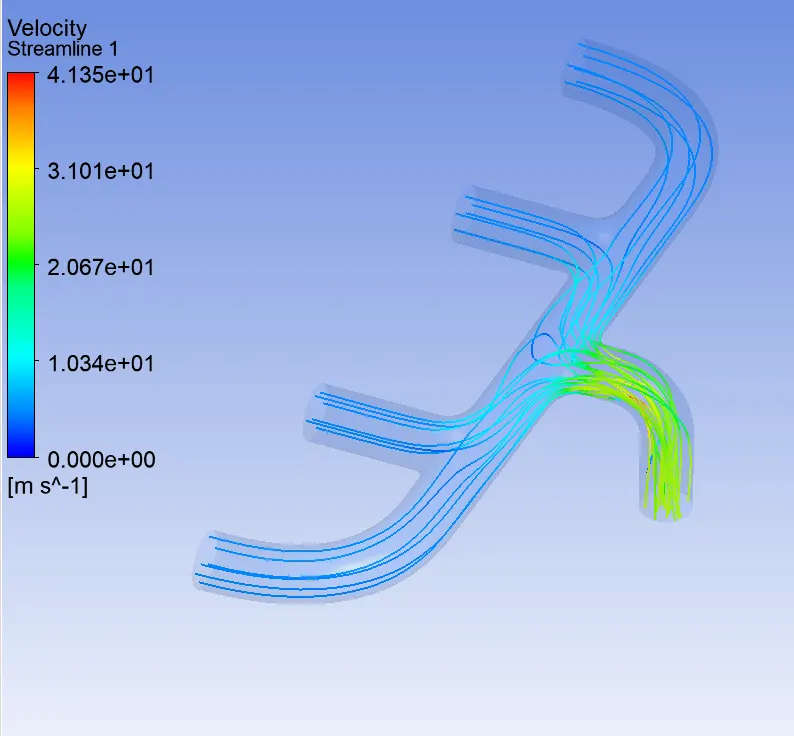
velocity streamlined plot

In the Analysis, the heat transfer coefficient obtained is of h=25 w/m^2k

Analytical solution:-

By using the Dittus Bolter relation

`Nu underset(D)() = 0.023*Re^(4/5)*Pr^n`

here n=0.3; Dia of the pipe(D)=0.166m

The Reynolds number of the flow is of Re = 56867.66

Prandtl No=`(mu*Cunderset(p)())/(k)`=0.744

Nussett number is calcuated as

`=0.023*56867.66^(4/5)*0.744^0.3 implies 158.8`

Nusselt No`(Nu underset(d)())=(hd)/k` =158.8

h=23.7w/m^2k.

Conclusions:

• The comparison between the theoretical and computational values of the thermal specific heat transfer coefficient yielded a close match, with both values being approximately 23.8 and 25 W/m^2K, respectively.
• The heat transfer coefficient value is concentrated in the immediate vicinity of the wall, allowing for the selection of y+ = 1 as the appropriate turbulence model.
• Evident boundary layer presence near the inlet indicated dominant viscous forces, resulting in near-zero slip velocity at the wall. Meanwhile, near the outlet, higher velocities and Reynolds numbers were observed due to the presence of one outlet and four inlets.
• The turbulence model maintained the y+ value within the desired range of 1, which was validated through comparison with the analytical solution, yielding results close to each other.
• The heat transfer coefficient was found to be approximately 25 W/m^2K, in good agreement with the analytical value.