Week 4 - CHT Analysis on Exhaust port
Aim
The aim is to conduct a conjugate heat transfer analysis on an exhaust port to calculate the wall/surface heat transfer coefficient.
Theory
Conjugate heat transfer analysis allows the heat transfer simulation between Solid and Fluid domains by exchanging thermal energy at the interfaces between them.
A CHT analysis, or Conjugate Heat Transfer analysis, is used in various fields and industries where understanding the combined effects of fluid flow and heat transfer is crucial. For example in heat exchangers, electronics cooling, gas turbines and engines etc.
Workflow
Geometry
The geometry of the exhaust port was opened in the spaceclaim and the fluid domain was extracted. (Prepare -> Volume extract -> Select the edges of the boundary -> click apply)
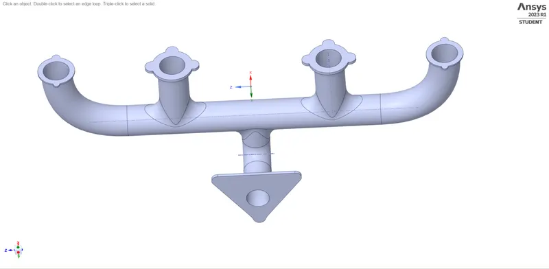
Now I extracted the fluid domain from the solid geometry which is shown in the above figure using the volume extract tool.
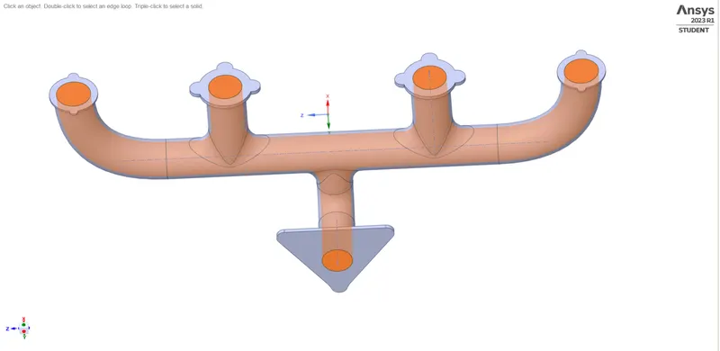
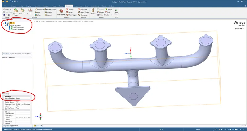
CHT analysis requires both the solid and the liquid domain, So both the solid volume and liquid volume are added as a single component and share topology is created in order to share the information between fluid and solid domains.
Mesh
At first, the named selection was given as follows.
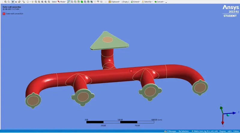
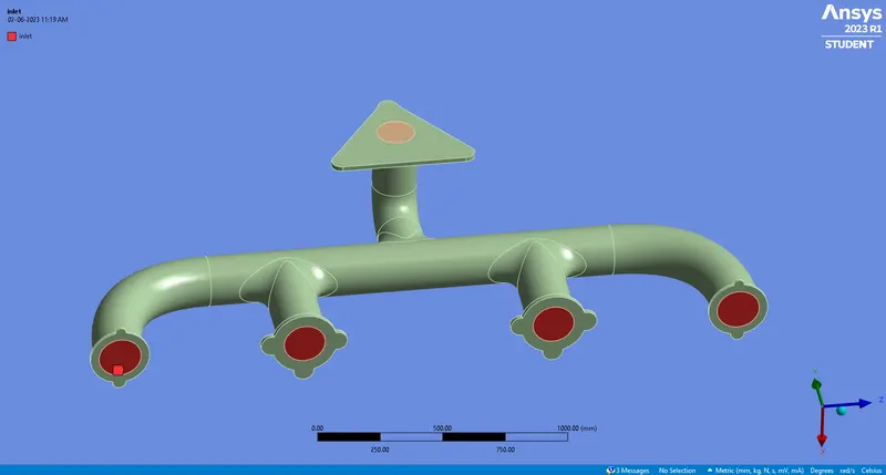
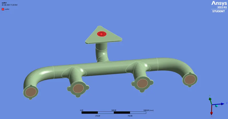
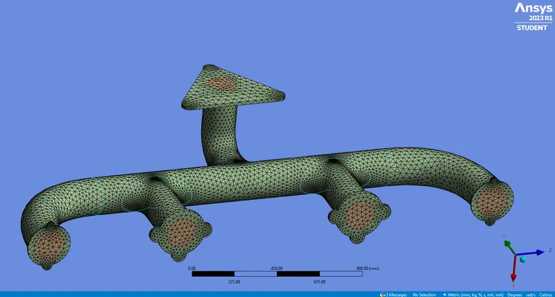
Initially, the default coarse mesh size was used and the mesh is generated (later mesh is refined).
Setup - Fluent
The mesh is updated and the fluent solver is opened. Here pressure-based solver is used and steady-state simulation is assumed.
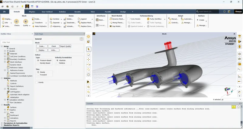
Setting up the model now:
The energy equation is turned on and the k-epsilon turbulence model has been selected.
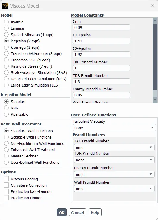
Material selection:
Fluid = Air
Solid = Aluminium
Boundry conditions:
Inlet - velocity = 5 m/s, temperature = 700k
Outlet - 0 Guage pressure
Wall - Convection is selected - heat transfer coefficient = 20 W/m^2k
Analytical calculation
Reynolds number
Re = (Density * flow speed * diameter of pipe)/Dynamic viscosity
Re = (1.225*5*0.166)/1.78e-5
Re = 56820.7
Prandtl Number
Pr = (specific heat * Dynamic viscosity)/Thermal conductivity
Pr = (1006.43*1.78e-5)/0.0242
Pr = 0.7442
Nusselt Number
Nu = 0.023*Re^0.8*Pr^0.3
Nu = 0.023*(56820.7)^0.8*(0.7442)^0.3
Nu = 133.91
Nu = (convective heat transfer coefficient * diameter of the pipe) / Thermal conductivity
From this equation, the convective heat transfer coefficient can be obtained.
Convective heat transfer coefficient = (133.91 * 0.0242)/0.166
Convective heat transfer coefficient = 19.523 Wm^-2K^-1
In our simulation, we have used the Convective heat transfer coefficient as 20 Wm^-2K^-1
Intialization
As a next step, the area-weighted average of the surface heat transfer coefficient for the internal surface of the pipeline is defined. After Hybrid initialization, the temperature contour and the animation contour are created.
Running the simulation
The simulation is set to run for 150 iterations
Results - Post-processing
We can observe the heat transfer coefficient plot and temperature contour plot
Results for baseline simulation
Temperature contour
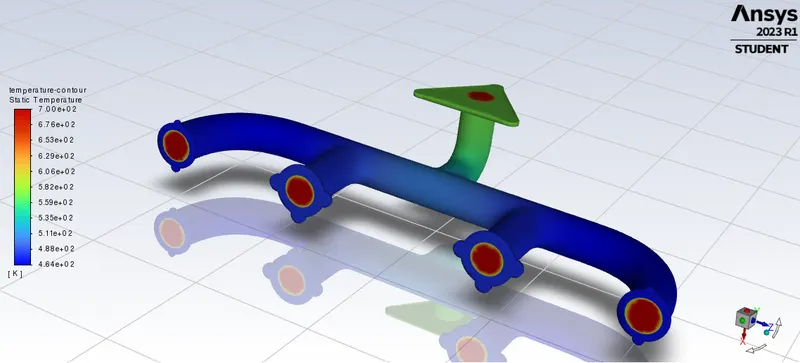
Surface heat transfer coefficient on the internal solid surface
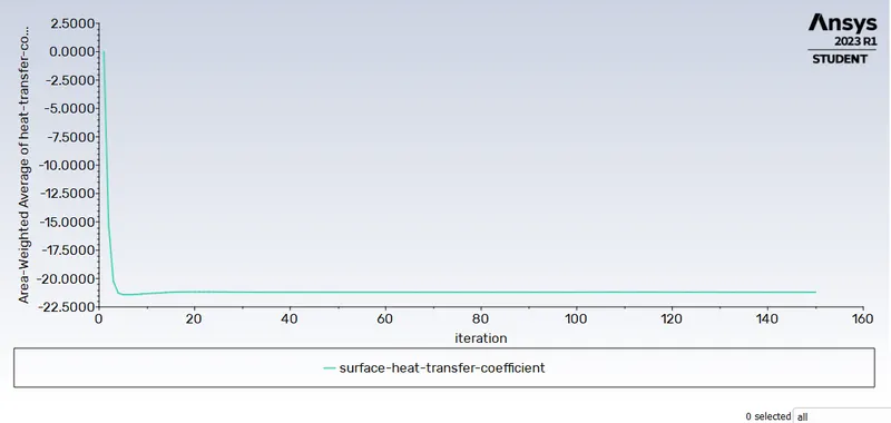
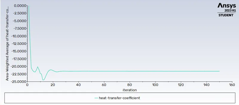
From the simulation, the Surface heat transfer coefficient on the internal solid surface is -21.19 Wm^-2K^-1
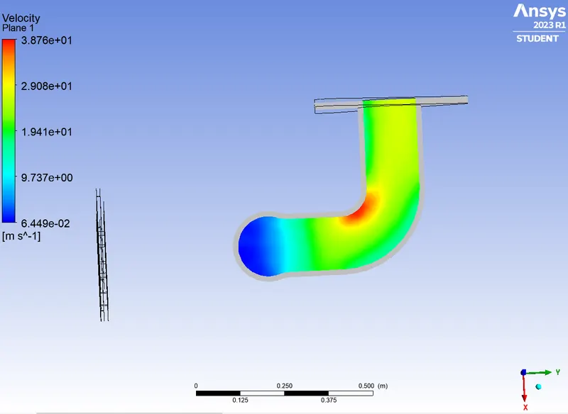
Velocity stream line plot: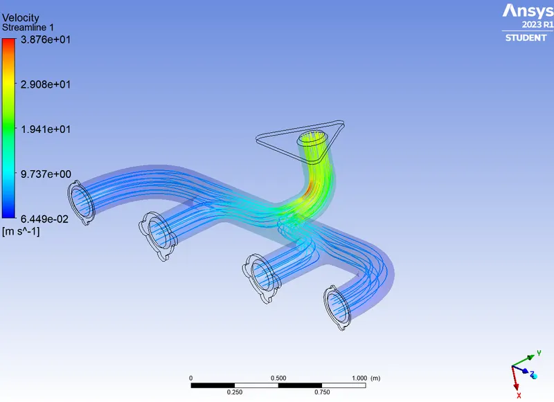
velocity plot
Now doing the Refined mesh (K epsilon model)
Geometry
As we have done earlier the geometry was imported to SpaceClaim and the fluid domain was extracted.
Meshing
An inflation layer was created. The mesh size of the fluid domain is kept to 20 mm. The inflation layer values are calculated for the y+ value of 30. We can find the value of the first layer thickness either manually or using online calculators. Using the online calculator the First wall thickness was found to be 3mm.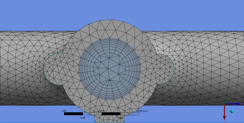
Setup - Fluent solver
All the materials and boundary conditions were the same. Just as in the last simulation, we ran the simulation for 150 iterations
Results- Refined mesh K epsilon model
Surface heat transfer coefficient on the internal surface plot
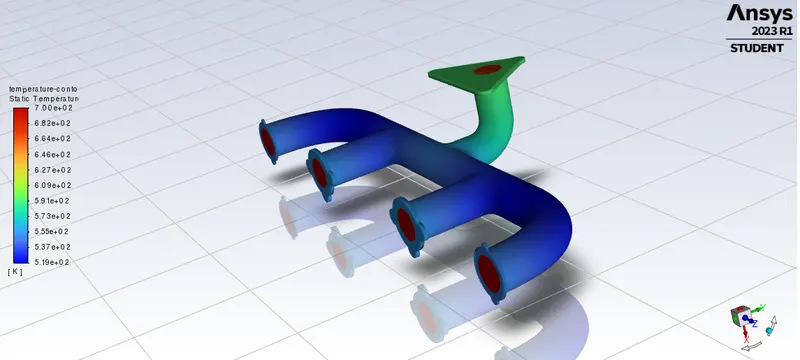
Temperature contour plot
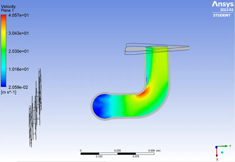
Velocity contour plot
Velocity streamline plot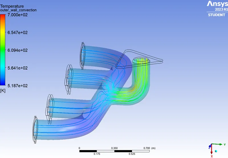
Refined mesh (k omega model)
Geometry
The same was before geometry was imported and fluid domain was extracted.
Meshing
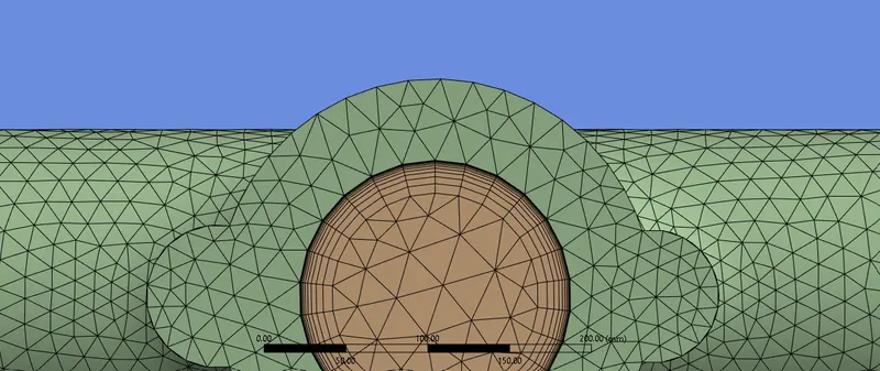
Meshing was done keeping the same y+ value at 3 and the corresponding first layer thickness was calculated.
Solving
The difference from the previous case is that here k omega model is selected.
Result
Surface heat transfer coefficient on the internal surface plot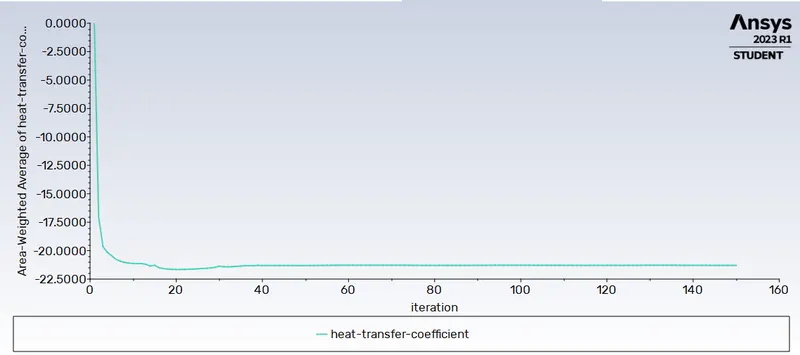
Temperature contour plot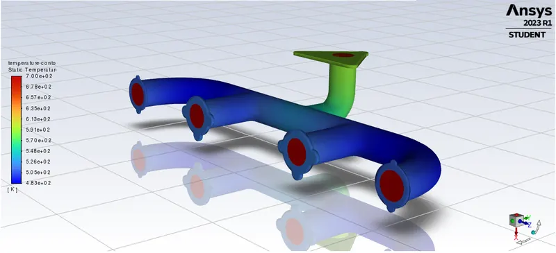
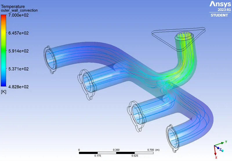
Velocity stream line plot
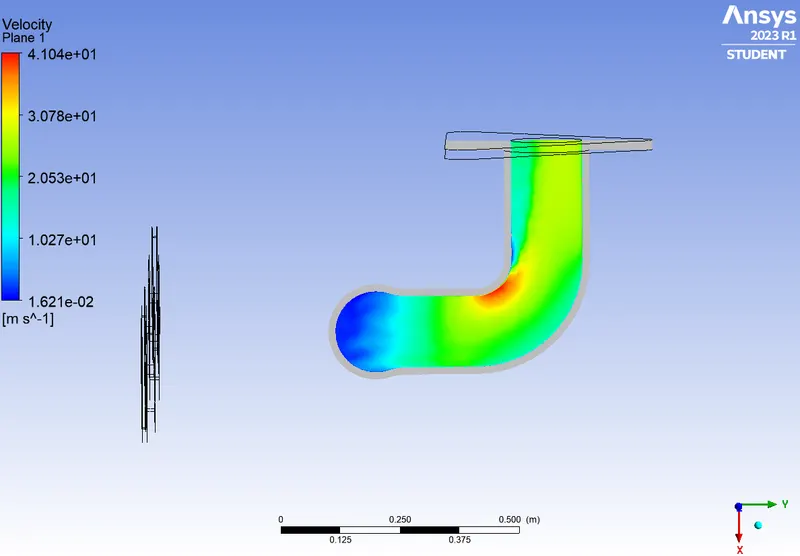
Velocity contour plot
Conclusion
The wall heat transfer coefficient observed is maximum at the outlet, where the velocity is maximum. As the air is being supplied through four inlets at the same velocity, and there is only one outlet, the velocity at the outlet is higher because of mass conservation. Specifically, by observing the velocity contour plots, we can see that the highest velocity is observed at the bend, and the highest heat transfer coefficient is also observed at the same position. This is because, at high velocity, the Reynolds number at that region will be higher and hence the heat transfer coefficient will also be higher.
The predicted HTC value was verified using the analytical method. The accuracy of heat transfer coefficient depends upon the selection of the turbulence model and the selection of the y+ value.